
wex is an R package for computing exact observation
weights for the Kalman filter and smoother, following Koopman and Harvey
(2003). The package provides tools for analyzing linear Gaussian
state-space models by quantifying how individual observations contribute
to filtered and smoothed state estimates.
These weights are particularly useful in applications such as dynamic factor models, where they can be used to decompose latent factors into contributions from observed variables (see Example 2 below).
The stable version of wex can be installed from
CRAN:
install.packages("wex")The development version of wex can be installed from GitHub:
# install.packages("devtools")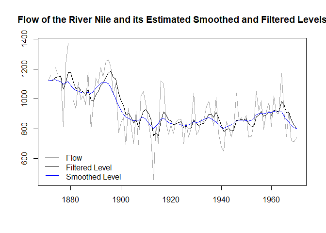
devtools::install_github("timginker/wex")In this illustrative example, we fit a local level model to the
Nile data and compute the corresponding filtered and
smoothed state estimates. We then extract the observation weights and
use them to reconstruct these estimates from the observed data.
The resulting estimates are shown in the plot below.
To illustrate the weight decomposition, consider the estimate of the local level at time \(t = 50\). Koopman and Harvey (2003) showed that the smoothed estimate \(\alpha_{t \mid T}\) can be expressed as
\[ \alpha_{t \mid T} = \sum_{j=1}^{T} w_j(\alpha_{t \mid T}) y_j, \]
where \(w_j(\alpha_{t \mid T})\)
denotes the observation weight assigned to \(y_j\). Missing values (NA) may
be present in the data; in such cases, the corresponding weights are set
to zero.
Similarly, the filtered estimate can be written as
\[ \alpha _{t|t}=\sum_{j=1}^{t}w_{j}(\alpha _{t|t})y_{j}. \]
We can compute the weight assigned to each observation using the
wex function and compare the resulting weighted averages
with the corresponding estimates obtained from the Kalman filter and
smoother.
wts <- wex(Tt=matrix(1),
Zt=matrix(1),
HHt = matrix(1385.066),
GGt = matrix(15124.13),
yt = t(y),
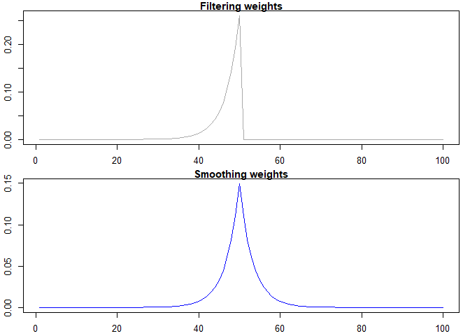
t=50)We can also visualize the weights assigned to each observation.
par(mfrow = c(2, 1),
    mar = c(2.2, 2.2, 1, 1),
    cex = 0.8)
plot(
  wts$Wt,
  col = "darkgrey",
  xlab = "",
  ylab = "",
  lwd = 1.5,
  type="l",
  main="Filtering weights"
)
plot(
  wts$WtT,
  col = "blue",
  xlab = "",
  ylab = " ",
  lwd = 1.5,
  type="l",
  main="Smoothing weights"
)
Finally, we verify that the filtered and smoothed estimates obtained from the Kalman filter coincide with those computed using the observation weights.
cat(
  "\nSmoothed level computed using the weights = ",
  sum(y * as.numeric(wts$WtT), na.rm = TRUE),
  "\nSmoothed level from the Kalman smoother = ",
  fit_ks$ahatt[50]
)
#>
#> Smoothed level computed using the weights =  834.9828
#> Smoothed level from the Kalman smoother = 834.9828cat(
"\nFiltered level computed using the weights = ",
sum(y * as.numeric(wts$Wt), na.rm = TRUE),
"\nFiltered level from the Kalman filter = ",
fit_kf$att[50]
)
#>
#> Filtered level computed using the weights = 849.307
#> Filtered level from the Kalman filter = 849.307In this example, we show how to compute observation weights in a dynamic factor model (DFM) and use them to decompose the latent factor into contributions from individual variables.
More formally, let \(x_t = (x_{1,t}, x_{2,t}, \dots, x_{n,t})^{\prime}\), for \(t = 1, 2, \dots, T\), denote a vector of \(n\) monthly series that have been transformed to achieve stationarity and standardized. A dynamic factor model assumes that \(x_t\) can be decomposed into two unobserved orthogonal components representing common and idiosyncratic factors. The model is given by
\[ x_t = \Lambda F_t + \varepsilon_t, \hspace{2pt} \varepsilon_t \sim N(0, R), \]
where \(F_t\) is an \((r \times 1)\) vector of unobserved common factors, \(\Lambda\) is an \((n \times r)\) matrix of factor loadings, and \(\varepsilon_t\) is an \((n \times 1)\) vector of idiosyncratic components. The common factors are assumed to follow the stationary VAR(\(p\)) process
\[ F_t = \sum_{s=1}^{p} \Phi_s F_{t-s} + u_t, \hspace{2pt} u_t \sim N(0, Q), \]
where \(\Phi_s\) are \((r \times r)\) matrices of autoregressive coefficients. Estimation and signal extraction can then be carried out using standard Kalman filtering and smoothing methods.
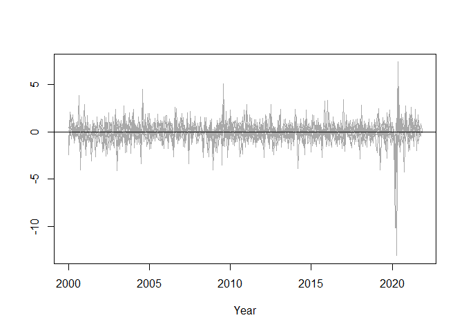
In this illustrative example, we use a dataset containing 10 monthly economic indicators spanning January 2000 to November 2021. All variables have been log-differenced, when necessary, to achieve stationarity. We assume a single latent factor following an AR(1) process.
The standardized data series and the corresponding smoothed factor estimate are shown in the plot below.
# Use the indicators dataset from wex
df <- scale(wex::indicators[,-1])

# Define the state-space matrices
Zt <- matrix(c(0.37873307, 0.37438154, 0.37767322,
                 0.02433999, 0.36020426, 0.23031769,
                 0.36584474, 0.35066644, 0.33420247,
                 0.01379571),
          ncol=1
)

Tt <- matrix(-0.3676422)

HHt <- matrix(1)

GGt <- matrix(c(
  0.7891011, 0, 0, 0, 0, 0, 0, 0, 0, 0,
  0, 0.3235747, 0, 0, 0, 0, 0, 0, 0, 0,
  0, 0, 0.7673983, 0, 0, 0, 0, 0, 0, 0,
  0, 0, 0, 0.01704776, 0, 0, 0, 0, 0, 0,
  0, 0, 0, 0, 0.9979156, 0, 0, 0, 0, 0,
  0, 0, 0, 0, 0, 0.8496217, 0, 0, 0, 0,
  0, 0, 0, 0, 0, 0, 0.8132641, 0, 0, 0,
  0, 0, 0, 0, 0, 0, 0, 0.9084006, 0, 0,
  0, 0, 0, 0, 0, 0, 0, 0, 0.7601053, 0,
  0, 0, 0, 0, 0, 0, 0, 0, 0, 0.1789897
), nrow = 10, ncol = 10, byrow = TRUE)

# Computing the smoothed values of the latent factor

fit_kf <- fkf(a0 = 0,
              P0 = diag(1e6, 1),
              dt = matrix(0,1),
              ct = rep(0,ncol(df)),
              Tt = Tt,
              Zt = Zt,
              HHt = HHt,
              GGt = GGt,
              yt = t(df))

fit_ks <- fks(fit_kf)


df.ts <- ts(df,start=c(2000,1),frequency = 12)
f_t <- ts(fit_ks$ahatt[1,])
tsp(f_t) <- tsp(df.ts)


plot(df.ts,plot.type = "single",col="darkgrey",xlab="Year",ylab="")
abline(h=0,lty=1)
lines(f_t, col="blue")
legend(
  "bottomleft",
  legend = c("Standardized series", "Smoothed factor estimate"),
  lwd = c(1, 1),
  col = c("darkgrey", "blue"),
  bty = "n"
)
We now use the wex function to decompose the final
estimate of the latent factor into contributions from each observed
variable.
# Extract weights for the final observation
wts <- wex(Tt=Tt,
        Zt=Zt,
        HHt = HHt,
        GGt = GGt,
        yt = t(df),
        t=nrow(df))
# Compute contributions

# Extract smoothing weights corresponding to the target state
sweights <- t(wts$WtT[1, , ])
colnames(sweights) <- colnames(df)

# Compute variable contributions as weighted sums of the observed data
contributions <- colSums(sweights * df, na.rm = TRUE)
The contributions are summarized in the Table below:
| Variable | Contribution |
|---|---|
| Total industrial production in Israel | 0.044 |
| Trade revenue | 0.065 |
| Service revenue | -0.023 |
| Employment (excluding absent workers) | 0.060 |
| Exports of services | 0.010 |
| Building starts | 0.001 |
| Imports of consumer goods | 0.019 |
| Imports of production inputs | 0.010 |
| Exports of goods | 0.003 |
| Job openings | -0.002 |
| Total | 0.188 |
The package supports two computational backends:
Koopman, S. J., and Harvey, A. C. (2003). Computing observation weights for signal extraction and filtering. Journal of Economic Dynamics and Control, 27(7), 1317–1333. https://doi.org/10.1016/S0165-1889(02)00061-1
Helske, J. (2017). KFAS: Exponential Family State Space Models in R. Journal of Statistical Software, 78(10), 1–39. https://doi.org/10.18637/jss.v078.i10
The views expressed here are solely of the author and do not necessarily represent the views of the Bank of Israel.
Please note that wex is still under development and may
contain bugs or other issues that have not yet been resolved. While we
have made every effort to ensure that the package is functional and
reliable, we cannot guarantee its performance in all situations.
We strongly advise that you regularly check for updates and install any new versions that become available, as these may contain important bug fixes and other improvements. By using this package, you acknowledge and accept that it is provided on an “as is” basis, and that we make no warranties or representations regarding its suitability for your specific needs or purposes.