cranDownloads()
from = and to = (use one
without other)pro.mode = TRUE shortcut to
cranlogs::cran_downloads()plot(cranDownloads())
packageRank()
plot(packageRank())
packageLog()
plot(packageLog())
cranDistribution()
package = NULLplot(cranDistribution())
package
argumentpackageHistory()
queryCount(), queryPackage(),
queryPercentile(), and queryRank()cranDownloads() (and ‘cranlogs’ package)
cranDownloads())
logInfo() checks availability and status of logs and
‘cranlogs’To install ‘packageRank’ from CRAN:
install.packages("packageRank")To install the development version (GitHub):
# You may need to install.packages("remotes").
remotes::install_github("lindbrook/packageRank", build_vignettes = TRUE)cranDownloads()cranDownloads() essentially uses all the same arguments
as cranlogs::cran_downloads():
cranlogs::cran_downloads(packages = "HistData")> date count package
> 1 2020-05-01 338 HistDataOther than the use of the singular for the ‘package’ argument, he
difference is that cranDownloads() adds five features:
cranDownloads(package = "GGplot2")## Error in cranDownloads(package = "GGplot2") :
## GGplot2: misspelled or not on CRAN.cranDownloads(package = "ggplot2")> date package count cumulative
> 1 2020-05-01 ggplot2 56357 56357
Note that this also works for inactive or “retired” packages in
the Archive:
With cranlogs::cran_downloads(), you specify a time
frame using the from and to arguments. The
downside is that you need to specify dates as “yyyy-mm-dd”. For
convenience’s sake, cranDownloads() allows you to use
“yyyy-mm” or yyyy (“yyyy” also works).
With cranlogs::cran_downloads(), if you want the
download counts for ‘HistData’ for
February 2020 you’d have to type out the whole date and remember that
2020 was a leap year:
cranlogs::cran_downloads(package = "HistData", from = "2020-02-01",
  to = "2020-02-29")
With cranDownloads(), you can just specify the
year and month:
cranDownloads(package = "HistData", from = "2020-02", to = "2020-02")With cranlogs::cran_downloads(), if you want the
download counts for ‘rstan’ for 2020
you’d type something like:
cranlogs::cran_downloads(packages = "rstan", from = "2022-01-01",
  to = "2022-12-31")
With cranDownloads(), you can use:
cranDownloads(package = "rstan", from = 2020, to = 2020)Note that “2020” will also work.
from = and to = in
cranDownloads()These additional date formats also provide convenient shortcuts.
Let’s say you want the year-to-date download counts for ‘rstan’. With
cranlogs::cran_downloads(), you’d type something like:
cranlogs::cran_downloads(package = "rstan", from = "2023-01-01",
  to = Sys.Date() - 1)
With cranDownloads(), you can just pass the
current year to from argument:
cranDownloads(package = "rstan", from = 2023)If you wanted the entire download history, pass the current year to
the to argument:
cranDownloads(package = "rstan", to = 2026)Note that the Posit/RStudio logs begin on 01 October 2012.
cranDownloads(package = "HistData", from = "2019-01-15", to = "2019-01-35")## Error in resolveDate(to, type = "to") : Not a valid date.By default, cranDownloads() also computes the cumulative
download count. This is useful for plotting growth curves.
cranDownloads(package = "HistData", when = "last-week")> date package count cumulative
> 1 2020-05-01 HistData 338 338
> 2 2020-05-02 HistData 259 597
> 3 2020-05-03 HistData 321 918
> 4 2020-05-04 HistData 344 1262
> 5 2020-05-05 HistData 324 1586
> 6 2020-05-06 HistData 356 1942
> 7 2020-05-07 HistData 324 2266Some of these features come at a cost: a one-time, per session
download of additional data. While those data are cached via the
‘memoise’ package, this adds time the first time
cranDownloads() is run.
For faster results, you can bypass those features by setting
pro.mode = TRUE. The downside is that you might see odd
results like zero downloads for packages on dates before they were on
CRAN or zero downloads for mis-spelled/non-existent packages. You’ll
also won’t be able to use the to argument by itself.
For example, ‘packageRank’ was first published on CRAN on 2019-05-16
- you can verify this via packageHistory("packageRank").
But if you use cranlogs::cran_downloads() or
cranDownloads(pro.mode = TRUE) before that date, you’ll see
zero downloads for days before 2019-05-16:
cranDownloads("packageRank", from = "2019-05-10", to = "2019-05-16", pro.mode = TRUE)
>         date     package count cumulative
> 1 2019-05-10 packageRank     0          0
> 2 2019-05-11 packageRank     0          0
> 3 2019-05-12 packageRank     0          0
> 4 2019-05-13 packageRank     0          0
> 5 2019-05-14 packageRank     0          0
> 6 2019-05-15 packageRank     0          0
> 7 2019-05-16 packageRank    68         68
This is particularly noticeable if you mis-spell or pass a “newer” package to cranDownloads().
cranDownloads("vr", from = "2019-05-10", to = "2019-05-16", pro.mode = TRUE)
>         date package count cumulative
> 1 2019-05-10      vr     0          0
> 2 2019-05-11      vr     0          0
> 3 2019-05-12      vr     0          0
> 4 2019-05-13      vr     0          0
> 5 2019-05-14      vr     0          0
> 6 2019-05-15      vr     0          0
> 7 2019-05-16      vr     0          0
Finally, if you just use to without a value for
from, you’ll get an error:
cranDownloads(to = 2024, pro.mode = TRUE)Error: You must also provide a date for "from".plot(cranDownloads())‘packageRank’ uses R’s generic plot method:
plot(cranDownloads(package = "HistData", from = "2019", to = "2019"))
If you pass a vector of package names for a single day, you’ll get a dotchart:
plot(cranDownloads(package = c("ggplot2", "data.table", "Rcpp"),
  from = "2020-03-01", to = "2020-03-01"))
If you pass a vector package names for multiple days, you’ll get a single graph with multiple time series plots using ‘ggplot2’ facets:
plot(cranDownloads(package = c("ggplot2", "data.table", "Rcpp"),
  from = "2020", to = "2020-03-20"))
To plot these data in a single plot frame, set
multi.plot = TRUE:
plot(cranDownloads(package = c("ggplot2", "data.table", "Rcpp"),
  from = "2020", to = "2020-03-20"), multi.plot = TRUE)
To plot these data as separate plots, on the same scale, set
graphics = "base". You’ll be prompted for each plot:
# Code only. Graph not shown.
plot(cranDownloads(package = c("ggplot2", "data.table", "Rcpp"), from = "2020",
  to = "2020-03-20"), graphics = "base")
To do the above using separate, independent scales, set
same.xy = FALSE:
# Code only. Graph not shown.
plot(cranDownloads(package = c("ggplot2", "data.table", "Rcpp"), from = "2020",
  to = "2020-03-20"), graphics = "base", same.xy = FALSE)
log.y = TRUETo use the base 10 logarithm of the download count in a plot, set
log.y = TRUE:
plot(cranDownloads(package = "HistData", from = "2019", to = "2019"),
  log.y = TRUE)
Note that any zero counts will be replaced by ones so that the
logarithm can be computed (This does not affect the data returned by
cranDownloads()).
package = NULLThe default first argument of cranDownloads() is
package = NULL. This computes the total number of package
downloads from CRAN. To plot these data, use:
plot(cranDownloads(from = 2019, to = 2019))
package = "R"cranDownloads(package = "R") computes the total number
of downloads of the R application by platfrom: “mac” = macOS, “src” =
source, and “win” = Windows. Note that, as with
cranlogs::cran_downloads(), you can only use “R”
or a vector of packages names, not both!.
To plot these data:
plot(cranDownloads(package = "R", from = 2019, to = 2019))
If you want plot the total count of R downloads, set
r.total = TRUE:
plot(cranDownloads(package = "R", from = 2019, to = 2019), r.total = TRUE)smooth = TRUETo add a smoother, use smooth = TRUE:
plot(cranDownloads(package = "rstan", from = "2019", to = "2019"),
  smooth = TRUE)
Note that loess is the default smoother, but with base graphics,
lowess is used when there are 7 or fewer observations. To control the
degree of smoothness, use the span argument (the default is
span = 0.75) for loess and where applicable, use the f
argument (the default is f = 2/3):
plot(cranDownloads(package = c("HistData", "rnaturalearth", "Zelig"),
  from = "2020", to = "2020-03-20"), smooth = TRUE, span = 0.75)

plot(cranDownloads(package = c("HistData", "rnaturalearth", "Zelig"),
  from = "2020", to = "2020-03-20"), smooth = TRUE, graphics = "ggplot2",
  span = 0.33)
se = TRUEWith graphs that use ‘ggplot2’, se = TRUE will add
confidence bands:
plot(cranDownloads(package = c("HistData", "rnaturalearth", "Zelig"),
  from = "2020", to = "2020-03-20"), smooth = TRUE, se = TRUE)
package.version = TRUE
or package.version = "line"To annotate a graph with a package’s release dates as ticks on the
top axis, set package.version = TRUE:
plot(cranDownloads(package = "rstan", from = "2019", to = "2019"),
  package.version = TRUE, unit.observation = "week")
If you want a vertical line, set
package.version = "line"
plot(cranDownloads(package = "rstan", from = "2019", to = "2019"),
  package.version = "line", unit.observation = "week")
r.version = TRUE
or r.version = “line”To annotate a graph with R release dates:
plot(cranDownloads(package = "rstan", from = "2019", to = "2019"),
  r.version = TRUE, unit.observation = "week")
If you want a vertical line, set
package.version = "line"
chatgpt = TRUE or
chatgpt = "line"By default, graphs that include ChatGPT’s release date, 2022-11-30, will be annotated with an axis tick and a vertical line:
plot(cranDownloads(package = "R", from = "2020-12", to = "2025-01"),
  r.total = TRUE, unit.observation = "week")
To exclude this, set plot.cranDownloads(chatgpt = FALSE)
weekend = TRUEWith unit.observation = "day" and
graphics = "base", you can highlight weekends, as empty
circles, by setting weekend = TRUE:
plot(cranDownloads(package = "rstan", from = "2024-06", to = "2024-06"),
  weekend = TRUE)
statistic = "cumulative"To plot growth curves using cumulative counts, set
statistic = "cumulative":
plot(cranDownloads(package = c("ggplot2", "data.table", "Rcpp"), from = "2020",
 to = "2020-03-20"), statistic = "cumulative", multi.plot = TRUE,
 points = FALSE)
The default unit of observation for cranDownloads() is
the day. The graph below plots the daily downloads for ‘cranlogs’ from
01 January 2022 through 27 September 2023.
plot(cranDownloads(package = "cranlogs", from = 2022, to = "2023-09-27"))
To view the data from a less granular perspective, change
plot.cranDownloads()’s unit.observation argument to “week”,
“month”, or “year”.
unit.observation = "week"The graph below plots the data aggregated by week, which begin on Sunday.
plot(cranDownloads(package = "cranlogs", from = 2022, to = "2023-09-27"),
  smooth = TRUE, unit.observation = "week")
Four things to note.
First, if the first week (far left) is incomplete (the ‘from’ date is not a Sunday), that observation will be split in two: one point for the observed total on ‘from’ date (empty gray square) and another point for the backdated total (blue asterisk). The backdated observation simply completes the week by pushing the start date back to include the previous Sunday.
In the example above, the nominal start date (01 January 2022) is pushed back to include data through the previous Sunday (26 December 2021). This is useful because when using a weekly unit of observation, the first “week” (far left) is often truncated. Consequently, you won’t get the most representative picture of the data. Backdating aims to fix this.
Second, if the last week (far right) is in-progress (the ‘to’ date is not a Saturday), that observation will be split in two: the observed total (empty gray square) and an estimated total based on the proportion of week completed (empty red circle).
Third, smoothers only use complete observations. This includes backdated data but excludes in-progress and estimated data.
Fourth, with the exception of first week’s observed count, which is plotted at its nominal date, points on the x-axis are plotted on Sundays.
unit.observation = "month"The graph below plots the data aggregated by month.
plot(cranDownloads(package = "cranlogs", from = 2022, to = "2023-09-27"),
  smooth = TRUE, unit.observation = "month")
Three things to note.
First, if the last/current month (far right) is still in-progress (it’s not yet the end of the month), that observation will be split in two: one point for the in-progress total (empty black square), another for the estimated total (empty red circle). The estimate is based on the proportion of the month completed. In the example above, the 635 observed downloads from April 1 through April 15 translates into an estimate of 1,270 downloads for the entire month (30 / 15 * 635).
Second, smoothers only use complete observations, not in-progress or estimated data.
Third, all points are plotted along the x-axis at the first day of the month.
Perhaps the biggest downside of using
cranDownloads(pro.mode = TRUE) is that you might draw
mistaken inferences from plotting the data since it can add false zeroes
to the data.
Using the example of ‘packageRank’, which was published on 2019-05-16:
plot(cranDownloads("packageRank", from = "2019-05", to = "2019-05",
  pro.mode = TRUE), smooth = TRUE)
plot(cranDownloads("packageRank", from = "2019-05", to = "2019-05",
  pro.mode = FALSE), smooth = TRUE)
packageRank()After spending some time with the nominal download counts above, the “compared to what?” question will come to mind. For instance, consider the data for the ‘cholera’ package from the first week of March 2020:
plot(cranDownloads(package = "cholera", from = "2020-03-01", to = "2020-03-07"))
Do Wednesday and Saturday reflect surges of interest in the package or surges of traffic to CRAN? To put it differently, how can we know if a given download count is typical or unusual?
To answer these questions, we can start by looking at the total number of package downloads:
plot(cranDownloads(from = "2020-03-01", to = "2020-03-07"))
Here we see that there’s a big difference between the work week and the weekend. This seems to indicate that the download activity for ‘cholera’ on the weekend seems high. Moreover, the Wednesday peak for ‘cholera’ downloads seems higher than the mid-week peak of total downloads.
One way to better address these observations is to locate your
package’s download counts in the overall frequency distribution of
download counts. ‘cholera’ allows you to do so via
cranDistribution(). Below are the distributions of
logarithm of download counts for Wednesday and Saturday. Each vertical
segment (along the x-axis) represents a download count. The height of a
segment represents that download count’s frequency. The location of ‘cholera’ in the
distribution is highlighted in red.
plot(cranDistribution(package = "cholera", date = "2020-03-04"))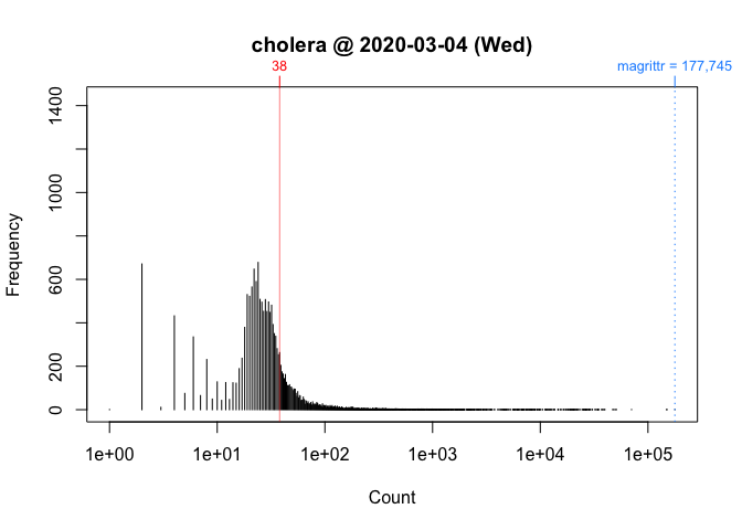
plot(cranDistribution(package = "cholera", date = "2020-03-07"))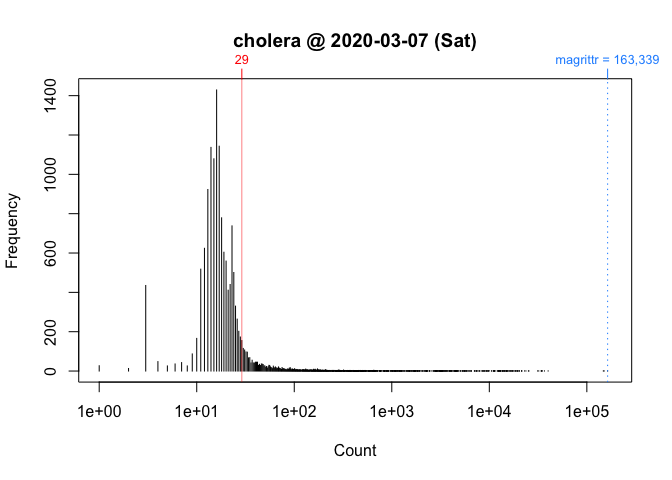
While these plots give us a better picture of where ‘cholera’ is located, comparisons between Wednesday and Saturday are still impressionistic: all we can confidently say is that the download counts for both days were greater than the mode.
To facilitate interpretation and comparison, I use the percentile rank of a download count instead of the simple nominal download count. This nonparametric statistic tells you the percentage of packages that had fewer downloads. In other words, it gives you the location of your package relative to the locations of all other packages. More importantly, by rescaling download counts to lie on the bounded interval between 0 and 100, percentile ranks make it easier to compare packages within and across distributions.
This function returns a package’s nominal count, rank, and percentile rank for a given day (default is “today” or last available).
For example, we can compare Wednesday (“2020-03-04”) to Saturday (“2020-03-07”):
packageRank(package = "cholera", date = "2020-03-04")
>         date package count            rank percentile
> 1 2020-03-04 cholera    38 5,788 of 18,038       67.9
On Wednesday, we can see that ‘cholera’ had 38 downloads, came in 5,788th place out of the 18,038 different packages downloaded, and earned a spot in the 68th percentile.
packageRank(package = "cholera", date = "2020-03-07")
>         date package count            rank percentile
> 1 2020-03-07 cholera    29 3,189 of 15,950         80
On Saturday, we can see that ‘cholera’ had 29 downloads, came in 3,189st place out of the 15,950 different packages downloaded, and earned a spot in the 80th percentile.
So contrary to what the nominal counts tell us, one could say that the interest in ‘cholera’ was actually greater on Saturday than on Wednesday.
To compute percentile ranks, I do the following. For each package, I tabulate the number of downloads and then compute the percentage of packages with fewer downloads. Here are the details using ‘cholera’ from Wednesday as an example:
pkg.rank <- packageRank(package = "cholera", date = "2020-03-04")

downloads <- pkg.rank$cran.data$count
names(downloads) <- pkg.rank$cran.data$package

round(100 * mean(downloads < downloads["cholera"]), 1)
> [1] 67.9
To put it differently:
(pkgs.with.fewer.downloads <- sum(downloads < downloads["cholera"]))
> [1] 12250

(tot.pkgs <- length(downloads))
> [1] 18038

round(100 * pkgs.with.fewer.downloads / tot.pkgs, 1)
> [1] 67.9Note that, by default, packageRank() computes the competition
rank (i.e., “1224”). Nominal
or ordinal ranking (i.e., “1234” ranking) is available by setting
packageRank(rank.ties = FALSE).
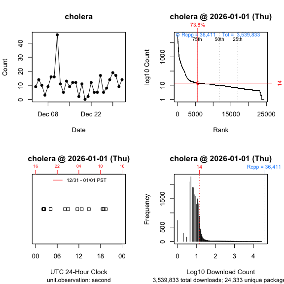
plot(packageRank())To visualize the results for packageRank() for Wednesday
and Sunday, use plot().
plot(packageRank(packages = "cholera", date = "2020-03-04"))
plot(packageRank(packages = "cholera", date = "2020-03-07"))
These graphs above, which are customized here to be on the same scale, plot the rank order of packages’ download counts (x-axis) against the logarithm of those counts (y-axis). It then highlights (in red) a package’s position in the distribution along with its percentile rank and download count. In the background, the 75th, 50th and 25th percentiles are plotted as dotted vertical lines. The package with the most downloads, ‘magrittr’ in both cases, is at top left (in blue). The total number of downloads is at the top right (in blue).
packageLog()This function returns the download log(s) for selected package(s) for a given day (the default is “today” or last available).
packageLog(package = "packageRank")> date time size r_version r_arch r_os package
> 1227088 2026-01-01 06:13:53 3285218 <NA> <NA> <NA> packageRank
> 1385514 2026-01-01 09:06:57 3501392 <NA> <NA> <NA> packageRank
> 26297 2026-01-01 09:26:58 3540287 <NA> <NA> <NA> packageRank
> 1897546 2026-01-01 10:01:27 3540380 <NA> <NA> <NA> packageRank
> 1897570 2026-01-01 10:01:29 3540380 <NA> <NA> <NA> packageRank
> 1899051 2026-01-01 10:03:51 2646084 <NA> <NA> <NA> packageRank
> 2166408 2026-01-01 10:05:46 2646087 <NA> <NA> <NA> packageRank
> 3256758 2026-01-01 11:07:30 3563240 <NA> <NA> <NA> packageRank
> 189598 2026-01-01 11:41:16 3560645 4.5.2 x86_64 mingw32 packageRank
> 1430170 2026-01-01 12:55:12 3560603 4.5.2 x86_64 mingw32 packageRank
> 2871829 2026-01-01 15:01:25 3560572 <NA> <NA> <NA> packageRank
> 665247 2026-01-01 18:58:57 3560623 4.5.2 x86_64 mingw32 packageRank
> 389617 2026-01-01 20:31:44 3539948 <NA> <NA> <NA> packageRank
> version country ip_id
> 1227088 0.8.3 US 1327
> 1385514 0.9.6 US 844
> 26297 0.9.7 US 407
> 1897546 0.9.7 US 1109
> 1897570 0.9.7 US 3749
> 1899051 0.9.7 US 770
> 2166408 0.9.7 US 770
> 3256758 0.9.7 US 855
> 189598 0.9.7 <NA> 2
> 1430170 0.9.7 <NA> 2
> 2871829 0.9.7 NL 7532
> 665247 0.9.7 <NA> 2
> 389617 0.9.7 US 129The logs record the “date”, “time”, “size” (in bytes), “r_version” (R version), “r_arch” (computer architecture: x86_64 = Intel, aarch64 = Apple Silicon, etc.), “r_os” (operating system: linux-gnu, darwin20, mingw32, etc.), “package”, “version” (package version), “country” (top level country code domain) and “ip_id” (anonymized IP address).
If you see information for “r_version”, “r_arch”, “r_os”, the client is the RStudio IDE. If those fields are NA, the client is something else (including Positron apparently).
plot(packageLog())Plotting the logs will give you time series plots. If you set
type = "1D"(1-dimensional), which is the default, you’ll
get a horizontal dot plot that shows the times when at least one
download is observed. If you set type = "2D"
(2-dimensional) you’ll get a time series graph that plots time versus
count. There are three time units: “second” (default), “minute”, and
“hour”.
The plot below contrasts the data with time unit “second” to the same data aggregated by time unit “hour”:
plot(packageLog(package = "cranlogs", date = "2026-01-01"), type = "1D",
  unit.observation = "second")
plot(packageLog(package = "cranlogs", date = "2026-01-01"), type = "1D",
  unit.observation = "hour")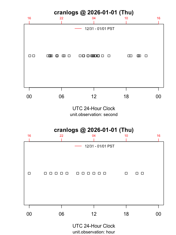
By default, your local time is appended to the top side of the graph
(side = 3). You can override this by either setting
local.timezone = FALSE to or by using a time zone from
OlsonNames(), e.g.,
local.timezone = "Australia/Sydney":
plot(packageLog(package = "HistData", date = "2026-01-01"), type = "2D",
  unit.observation = "hour")
plot(packageLog(package = "HistData", date = "2026-01-01"), type = "2D",
  unit.observation = "hour", local.timezone = "Australia/Sydney")
packageHistory()This function returns a package’s release history.
packageHistory(package = "cholera")
>    Package Version       Date Repository
> 1  cholera   0.2.1 2017-08-10    Archive
> 2  cholera   0.3.0 2018-01-26    Archive
> 3  cholera   0.4.0 2018-04-01    Archive
> 4  cholera   0.5.0 2018-07-16    Archive
> 5  cholera   0.5.1 2018-08-15    Archive
> 6  cholera   0.6.0 2019-03-08    Archive
> 7  cholera   0.6.5 2019-06-11    Archive
> 8  cholera   0.7.0 2019-08-28    Archive
> 9  cholera   0.7.5 2021-04-22    Archive
> 10 cholera   0.7.9 2021-10-11    Archive
> 11 cholera   0.8.0 2023-03-01    Archive
> 12 cholera   0.9.0 2025-03-14    Archive
> 13 cholera 0.9.1 2025-05-01 CRANcranDistribution()This function computes the frequency distribution of downloads and returns summary statistics and the top-N packages.
cranDistribution(package = NULL)> $date
> [1] "2026-01-01 Thursday"
>
> $unique.packages.downloaded
> [1] "24,333"
>
> $total.downloads
> [1] "3,539,833"
>
> $top.n
> package count rank nominal.rank percentile
> 1 Rcpp 36411 1 1 100.0
> 2 rlang 27090 2 2 100.0
> 3 cli 26311 3 3 100.0
> 4 jsonlite 24401 4 4 100.0
> 5 glue 24052 5 5 100.0
> 6 magrittr 23951 6 6 100.0
> 7 lifecycle 23228 7 7 100.0
> 8 dplyr 22980 8 8 100.0
> 9 R6 22700 9 9 100.0
> 10 withr 22484 10 10 100.0
> 11 vctrs 21936 11 11 100.0
> 12 systemfonts 21623 12 12 100.0
> 13 textshaping 21357 13 13 99.9
> 14 tibble 21324 14 14 99.9
> 15 pillar 20748 15 15 99.9
> 16 curl 20739 16 16 99.9
> 17 stringr 20060 17 17 99.9
> 18 purrr 19813 18 18 99.9
> 19 utf8 19337 19 19 99.9
> 20 fs 19284 20 20 99.9If you pass a package to the function, e.g.,
cranDistribution(package = "packageRank"), data for that
package will be appended:
cranDistribution(package = "packageRank")> $date
> [1] "2026-01-01 Thursday"
>
> $unique.packages.downloaded
> [1] "24,333"
>
> $total.downloads
> [1] "3,539,833"
>
> $top.n
> package count rank nominal.rank percentile
> 1 Rcpp 36411 1 1 100.0
> 2 rlang 27090 2 2 100.0
> 3 cli 26311 3 3 100.0
> 4 jsonlite 24401 4 4 100.0
> 5 glue 24052 5 5 100.0
> 6 magrittr 23951 6 6 100.0
> 7 lifecycle 23228 7 7 100.0
> 8 dplyr 22980 8 8 100.0
> 9 R6 22700 9 9 100.0
> 10 withr 22484 10 10 100.0
> 11 vctrs 21936 11 11 100.0
> 12 systemfonts 21623 12 12 100.0
> 13 textshaping 21357 13 13 99.9
> 14 tibble 21324 14 14 99.9
> 15 pillar 20748 15 15 99.9
> 16 curl 20739 16 16 99.9
> 17 stringr 20060 17 17 99.9
> 18 purrr 19813 18 18 99.9
> 19 utf8 19337 19 19 99.9
> 20 fs 19284 20 20 99.9
>
> $package.data
> package count rank nominal.rank percentile
> 7300 packageRank 13 7668 7300 68.5plot(cranDistribution())If you plot the above functions, you’ll get a histogram of the overall distribution of download counts (base 10 logarithm):
plot(cranDistribution(package = NULL))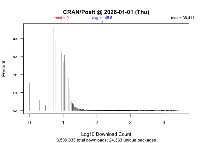
If you pass a package to the function, its location in the distribution will be annotated:
plot(cranDistribution(package = "packageRank"))plot(cranDistribution(package = "packageRank", date = "2026-01-01"))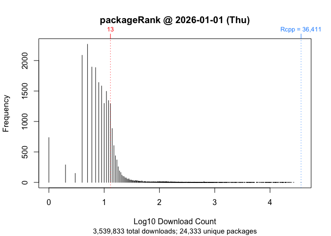
To do a reverse lookup (e.g., find packages with a given download
count or percentile rank), use queryCount(),
queryPackage(), queryPercentile() or
queryRank().
queryCount(count = 100)
>        package count rank nominal.rank percentile
> 1        ascii   100 2717         2710       89.9
> 2        gains   100 2717         2711       89.9
> 3      ipsRdbs   100 2717         2712       89.9
> 4      nhanesA   100 2717         2713       89.9
> 5       rxode2   100 2717         2714       89.9
> 6     sdcMicro   100 2717         2715       89.9
> 7       TOSTER   100 2717         2716       89.9
> 8 treesitter.r 100 2717 2717 89.9queryPackage(package = "cholera")
> package count rank nominal.rank percentile
> 1 cholera 19 4765 4656 82.2head(queryPercentile(percentile = 99))
> package count rank nominal.rank percentile
> 1 zip 18021 148 148 99.4
> 2 reshape2 17900 149 149 99.4
> 3 openxlsx 17715 150 150 99.4
> 4 cowplot 17423 151 151 99.4
> 5 doBy 17396 152 152 99.4
> 6 urca 17364 153 153 99.4Note that due to the discrete nature of counts, your choice of percentile may not be available. For details, see this note in the ‘packageRank’ GitHub repository.
queryRank(rank = 9)
>   package count rank nominal.rank percentile
> 1 glue 71506 9 9 100‘cranlogs’ computes package downloads by counting log entries. While straightforward, this approach can run into problems. Putting aside package dependencies (the effect of packages that use packages), what I have in mind here are two types of “invalid” log entries.
The first are software artifacts. These are entries that are smaller, often orders of magnitude smaller, than the package’s binary or source file. The second are behavioral artifact. The main culprit here appears to stem from efforts to download all of the packages on CRAN. In both cases, simple nominal counts will give you an inflated sense of the degree of interest in your package.
For what it’s worth, an early examination of inflation is included as part of this R-hub blog post.
When looking at package’s download logs, the first thing you’ll often see are wrongly sized log entries. They come in two flavors: 1) “small” entries approximately 500 bytes in size and 2) “medium” entries (i.e., “small” <= “medium” <= full download). “Small” entries manifest themselves as standalone entries, as paired with a full download, or as part of a triplet with a “medium” and a full download. “Medium” entries manifest themselves as either a standalone entry or as part of a triplet.
The example below illustrates a triplet:
packageLog(date = "2020-07-01")$cholera[4:6, -(4:6)]
>               date     time    size package version country ip_id
> 3998633 2020-07-01 07:56:15   99622 cholera   0.7.0      US  4760
> 3999066 2020-07-01 07:56:15 4161948 cholera   0.7.0      US  4760
> 3999178 2020-07-01 07:56:15     536 cholera   0.7.0      US  4760
The “medium” entry is the first observation (99,622 bytes). The full download is the second entry (4,161,948 bytes). The “small” entry is the last observation (536 bytes). At a minimum, what makes a triplet (or a pair) is that all members share system configuration (e.g. IP address, etc.) and have identical or adjacent time stamps.
To deal with “small” log entries, I filter out observations smaller than 1,000 bytes (the smallest package on CRAN appears to be ‘LifeInsuranceContracts’, whose source file weighs in at 1,100 bytes). “Medium” entries are harder to handle. I remove them using a function that looks up a package’s actual size.
The other pattern you’ll often see when looking at package download logs is the presence of “too many” prior versions. While there are legitimate reasons for downloading past versions (e.g., research, container-based software distribution, etc.), I’d argue that such patterns are “fingerprints” of efforts to download CRAN. While there is nothing inherently problematic about this (other than infrastructure costs), it does inflate your package download count. When your package is downloaded as part of such efforts, those downloads are more a reflection of an interest in CRAN itself (a collection of packages) rather than of an interest in your package per se.
To illustrate, consider the following example:
packageLog(package = "cholera", date = "2020-07-31")[8:14, -(4:6)]> date time size package version country ip_id
> 132509 2020-07-31 21:03:06 3797776 cholera 0.2.1 US 14
> 132106 2020-07-31 21:03:07 4285678 cholera 0.4.0 US 14
> 132347 2020-07-31 21:03:07 4109051 cholera 0.3.0 US 14
> 133198 2020-07-31 21:03:08 3766514 cholera 0.5.0 US 14
> 132630 2020-07-31 21:03:09 3764848 cholera 0.5.1 US 14
> 133078 2020-07-31 21:03:11 4275831 cholera 0.6.0 US 14
> 132644 2020-07-31 21:03:12 4284609 cholera 0.6.5 US 14Here, we see that seven different versions of the package were downloaded as a sequential bloc. A little digging shows that on that date there were seven extant versions of ‘cholera’:
packageHistory(package = "cholera")> Package Version Date Repository
> 1 cholera 0.2.1 2017-08-10 Archive
> 2 cholera 0.3.0 2018-01-26 Archive
> 3 cholera 0.4.0 2018-04-01 Archive
> 4 cholera 0.5.0 2018-07-16 Archive
> 5 cholera 0.5.1 2018-08-15 Archive
> 6 cholera 0.6.0 2019-03-08 Archive
> 7 cholera 0.6.5 2019-06-11 Archive
> 8 cholera 0.7.0 2019-08-28 CRANAnd such, it may be useful to exclude such entries. To do so, I filter out these entries in two ways. The first identify IP addresses that download “too many” packages and then filter out campaigns, large blocs of downloads that occur in (nearly) alphabetical order. The second looks for campaigns not associated with “greedy” IP addresses and filters out sequences of past versions downloaded in a narrowly defined time window.
To get an idea of how inflated your package’s download count may be,
use filteredDownloads(). Below are the results for
‘ggplot2’ for 15 September 2021.
filteredDownloads(package = "ggplot2", date = "2021-09-15")
>         date package downloads filtered.downloads delta inflation
> 1 2021-09-15 ggplot2    113842             108326  5516    5.09 %
While there were 113,842 nominal downloads, applying all the filters reduced that number to 111,662, an inflation of 1.95%.
There are 5 filters. You can control them using the following arguments (listed in order of application):
ip.filter: removes campaigns of “greedy” IP
addresses.small.filter: removes entries smaller than 1,000
bytes.sequence.filter: removes blocs of past versions.size.filter: removes entries smaller than a package’s
binary or source file.version.filter: include only the most recent package
version.For filteredDownloads(), they are all on by default. For
packageLog() and packageRank(), they are off
by default. To apply them, simply set the argument for the filter you
want to TRUE:
packageRank(package = "cholera", small.filter = TRUE)Alternatively, for packageLog() and
packageRank() you can simply set
all.filters = TRUE.
packageRank(package = "cholera", all.filters = TRUE)Note that the all.filters = TRUE is contextual.
Depending on the function used, you’ll either get the CRAN-specific or
the package-specific set of filters. The former sets
ip.filter = TRUE and size.filter = TRUE; it
works independently of packages at the level of the entire log. The
latter sets sequence.filter = TRUEandsize.filter TRUE`; it
relies on package specific information (e.g., size of source or binary
file).
Ideally, we’d like to use both sets. However, the package-specific
set is computationally expensive because they need to be applied
individually to all packages in the log, which can involve tens of
thousands of packages. While not unfeasible, currently this takes a long
time. For this reason, when all.filters = TRUE,
packageRank(), ipPackage(),
countryPackage(), countryDistribution() and
cranDistribution() use only CRAN specific filters while
packageLog(), packageCountry(), and
filteredDownloads() use both CRAN and package specific
filters.
To understand when results become available, you need to know that ‘packageRank’ has two upstream, online dependencies. The first is Posit/RStudio’s CRAN package download logs. These logs record traffic that passes through the “0-Cloud” mirror, which is currently sponsored by Posit. The second is Gábor Csárdi’s ‘cranlogs’ R package, which uses the Posit/RStudio logs to compute the download counts of both R packages and the R application itself.
The CRAN package download logs for the previous day are typically posted by 17:00 UTC. The results for ‘cranlogs’ usually become available soon thereafter.
Occasionally, problems with “today’s” data can arise due to problems with one or both of the upstream dependencies (illustrated below).
CRAN Download Logs --> 'cranlogs' --> 'packageRank'If there’s a problem with the logs (e.g., they’re not posted on time), both ‘cranlogs’ and ‘packageRank’ will be affected. If this happens, you’ll see things like an unexpected zero count(s) for your package(s) (actually, you’ll see a zero download count for both your package and for all of CRAN), data from “yesterday”, or a “Log is not (yet) on the server” error message.
'cranlogs' --> packageRank::cranDownloads()If there’s a problem with ‘cranlogs’ but
not with the logs, only
cranDownalods() will be affected. In that case, you might
get a warning that only “previous” results will be used. All other ‘packageRank’
functions should work since they either directly access the logs or use
some other data source. Usually, these errors resolve themselves the
next time the underlying scripts are run (tomorrow, if not sooner).
logInfo()To check the status of the download logs and ‘cranlogs’, use
logInfo(). This function checks whether 1) “today’s” log is
posted on Posit/RStudio’s server and 2) “today’s” results have been
computed by ‘cranlogs’.
logInfo()$`Today's log/result`
[1] "2023-02-01"
$`Today's log posted?`
[1] "Yes"
$`Today's results on 'cranlogs'?`
[1] "No"
$status
[1] "Today's log is typically posted by 01 Feb 09:00 PST -- 01 Feb 17:00 UTC."Because you’re typically interested in today’s log file, another thing that affects availability is your time zone. For example, let’s say that it’s 09:01 on 01 January 2021 and you want to compute the percentile rank for ‘ergm’ for the last day of 2020. You might be tempted to use the following:
packageRank(package = "ergm")However, depending on where you make this request, you may not get the data you expect. In Honolulu, USA, you will. In Sydney, Australia you won’t. The reason is that you’ve forgotten a key piece of trivia: Posit/RStudio typically posts yesterday’s log around 17:00 UTC the following day.
The expression works in Honolulu because 09:01 HST on 01 January 2021 is 19:01 UTC 01 January 2021. So the log you want has been available for 2 hours. The expression fails in Sydney because 09:01 AEDT on 01 January 2021 is 31 December 2020 22:01 UTC. The log you want won’t actually be available for another 19 hours.
To make life a little easier, ‘packageRank’ does two things. First, when the log for the date you want is not available (due to time zone rather than server issues), you’ll just get the last available log. If you specified a date in the future, you’ll either get an error message or a warning with an estimate of when the log you want should be available.
Using the Sydney example and the expression above, you’d get the results for 30 December 2020:
packageRank(package = "ergm")> date package count rank percentile
> 1 2020-12-30 ergm 292 878 of 20,077 95.6If you had specified the date, you’d get an additional warning:
packageRank(package = "ergm", date = "2021-01-01")> date package count rank percentile
> 1 2020-12-30 ergm 292 878 of 20,077 95.6
Warning message:
2020-12-31 log arrives in ~19 hours at 02 Jan 04:00 AEDT. Using previous!Keep in mind that 17:00 UTC is not a hard deadline. Barring server issues, the logs are usually posted a little before that time. I don’t know when the script starts but the posting time seems to be a function of the number of entries: closer to 17:00 UTC when there are more entries (e.g., weekdays); earlier than 17:00 UTC when there are fewer entries (e.g., weekends). Again, barring server issues, the ‘cranlogs’ results are usually available before 18:00 UTC.
Here’s what you might see using the Honolulu example:
logInfo(details = TRUE)$`Today's log/result`
[1] "2020-12-31"
$`Today's log posted?`
[1] "Yes"
$`Today's results on 'cranlogs'?`
[1] "Yes"
$`Available log/result`
[1] "Posit/RStudio (2020-12-31); 'cranlogs' (2020-12-31)."
$`Current date-time`
[1] "01 Jan 09:01 HST -- 01 Jan 19:01 UTC"
$status
[1] "Everything OK."The function uses your local time zone, which depends on R’s ability
to compute your local time and time zone (e.g., Sys.time()
and Sys.timezone()). My understanding is that there may be
operating system or platform specific issues that could undermine
this.
There are three data errors and one data issue to note. I’ve patched the errors.
The logs collected between late 2012 and the beginning of 2013 are a bit jumbled.
To understand the problem, we need to be know that the Posit/RStudio download logs are stored as separate files with a name/URL that embeds the log’s date:
http://cran-logs.rstudio.com/2022/2022-01-01.csv.gzFor the logs in question, this convention was broken in three ways: i) some logs are effectively duplicated (same log, different names), ii) at least one mislabeled log and iii) the logs from 13 October through 28 December are offset by +3 days (e.g., the file with the name/URL “2012-12-01” contains the log for “2012-11-28”). As a result, we get erroneous download counts and actually lose the last three logs of 2012. Details are available here.
Unsurprisingly, this affects download counts.
Functions that rely on cranlogs::cran_download() (e.g.,
‘packageRank::cranDownloads()’,
‘adjustedcranlogs’
and ‘dlstats’)
are susceptible to the first error - duplicate names. My understanding
is that this is because ‘cranlogs’ uses
the date in the log rather than the date in the filename/URL to retrieve
logs. To put it differently, ‘cranlogs’ can’t
detect multiple instances of logs with the same date. I found 3 logs
with duplicate filename/URLs, and 5 additional instances of overcounting
(including one of tripling). ‘fixCranlogs()’
addresses this overcounting by recomputing the download counts using the
correct log(s) when any of the eight problematic dates are requested.
Details about the 8 days and fixCranlogs() can be found here.
Functions that access logs via their filename/URL, e.g.,
packageRank() and packageLog(), are affected
by the second and third defects - mislabeled and offset logs. fixDate_2012()
addresses this by re-mapping problematic logs so that you get the log
you expect.
Typically, the pattern of R application downloads is a series of weekday peaks and weekends troughs. You can see this in the graph below, which plots the January 2022 data broken down by platform (Mac, Source, and Windows) and weekday/weekend (filled v. empty circles):
plot(cranDownloads(package = "R", from = "2022-01", to = "2022-01"),
  r.version = TRUE, weekend = TRUE)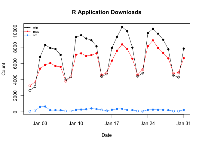
However, between November 2022 and March 2023, this pattern was broken. On Sundays (06 November 2022 - 19 March 2023) and Wednesdays (18 January 2023 - 15 March 2023), there were noticeable, repeated, orders-of-magnitude spikes in the daily downloads of just the Windows version of R.

These spikes appear to be real patterns in the data and not coding
errors. Detailed, visual evidence for this can be found online in this
note
in the packageRank GitHub respository.
From 2023-09-13 through 2023-10-02, the download counts for the R
application returned by
cranlogs::cran_downloads(package = "R"), is, with two
exceptions, twice the count you’d get when looking at the actual log(s).
The two exceptions are: 1) 2023-09-28 where the counts are identical but
for a “rounding error” possibly due to NAs and 2) 2023-09-30 where there
is actually a three-fold difference.
Here are the relevant ratios of counts comparing ‘cranlogs’ results with counts based on the underlying logs:
    2023-09-12 2023-09-13 2023-09-14 2023-09-15 2023-09-16 2023-09-17 2023-09-18 2023-09-19
osx          1          2          2          2          2          2          2          2
src          1          2          2          2          2          2          2          2
win          1          2          2          2          2          2          2          2
    2023-09-20 2023-09-21 2023-09-22 2023-09-23 2023-09-24 2023-09-25 2023-09-26 2023-09-27
osx          2          2          2          2          2          2          2          2
src          2          2          2          2          2          2          2          2
win          2          2          2          2          2          2          2          2
    2023-09-28 2023-09-29 2023-09-30 2023-10-01 2023-10-02 2023-10-03
osx   1.000000          2          3          2          2          1
src   1.000801          2          3          2          2          1
win   1.000000          2          3          2          2          1
Details and code for replication can be found in issue #69. fixRCranlogs()
corrects the problem. Note that there was a similar issue for package
download counts around the same period but that is now fixed in ‘cranlogs’. For
details, see issue #68
In 2025, 7 logs, 8/25-8/26 and 8/29-9/02, appear to be lost. For what it’s worth, both gaps were preceded by two unusually large number of downloads: Sun 8/24 (14,521,256) and Wed 8/27 & Thu 8/28 (16,860,505 and 16,477,023). These outliers are approximately twice the size of “typical” download counts (see graph below).
As a “fix”, the missing dates (see cholera::missing.date),
cranDownloads() does the following. First, when a missing
date is included it prints a message in the console. Second, when
plotting two gray polygons are added to the graph to highlight those
dates. They are labeled with a “⌀” (empty set) on the top axis. Third,
smoothers ignore the missing data.
The graph below, which plots the total number of downloads recorded by the Posit/RStudio mirror from Sat 7/05 through Sun 9/14, shows the magnitude of the outliers and the two graphical fixes (open circles are weekends).
plot(cranDownloads(from = "2025-07-05", to = "2025-09-10"), smooth = TRUE,
  points = TRUE, weekend = TRUE)
> Missing: 2025-08-25, 2025-08-26, 2025-08-29, 2025-08-30, 2025-08-31, 2025-09-01, 2025-09-02
This section describes some additional issues that may be of interest.
Note that the “raw” Bioconductor package download are already aggregated by month.
While the IP addresses in the Posit/RStudio logs are
anonymized, packageCountry() and
countryPackage() the logs include ISO country codes or top
level domains (e.g., AT, JP, US).
Note that coverage extends to only about 85% of observations (approximately 15% country codes are NA), and that there seems to be a a couple of typos for country codes: “A1” (A + number one) and “A2” (A + number 2). According to Posit/RStudio’s documentation, this coding was done using MaxMind’s free database, which no longer seems to be available and may be a bit out of date.
To avoid the bottleneck of downloading multiple log files,
packageRank() is currently limited to individual calendar
dates. To reduce the bottleneck of re-downloading logs, which can
approach 100 MB, ‘packageRank’
makes use of memoization via the ‘memoise’
package.
Here’s relevant code:
fetchLog <- function(url) data.table::fread(url)

mfetchLog <- memoise::memoise(fetchLog)

if (RCurl::url.exists(url)) {
  cran_log <- mfetchLog(url)
}

# Note that data.table::fread() relies on R.utils::decompressFile().
This means that logs are cached; logs that have already been downloaded in your current R session will not be downloaded again.
With R 4.0.3, the timeout value for internet connections became more explicit. Here are the relevant details from that release’s “New features”:
The default value for options("timeout") can be set from environment variable
R_DEFAULT_INTERNET_TIMEOUT, still defaulting to 60 (seconds) if that is not set
or invalid.
This change can affect functions that download logs. This is
especially true over slower internet connections or when you’re dealing
with large log files. To fix this, fetchCranLog() will, if
needed, temporarily set the timeout to 600 seconds.