Package {MGBT}

Type:	Package
Title:	Multiple Grubbs-Beck Low-Outlier Test
Version:	1.1.6
Depends:	R (≥ 4.0.0)
Suggests:	dataRetrieval, lmomco
Date:	2026-05-21
Description:	Compute the multiple Grubbs-Beck low-outlier test on positively distributed data and utilities for noninterpretive U.S. Geological Survey annual peak-streamflow data processing discussed in Cohn et al. (2013) and England et al. (2017) <doi:10.3133/tm4B5>. Other utilities for working with peak streamflow are provided.
Maintainer:	William H. Asquith <wasquith@usgs.gov>
License:	CC0
Copyright:	This software is in the public domain because it contains materials that originally came from the United States Geological Survey, an agency of the United States Department of Interior. For more information, see the official USGS copyright policy at https://www.usgs.gov/information-policies-and-instructions/copyrights-and-credits
NeedsCompilation:	no
URL:	https://doi.org/10.5066/P9CW9EF0
Packaged:	2026-05-26 21:54:54 UTC; wasquith
Author:	William H. Asquith [aut, cre], John F. England [aut, ctb], George R. Herrmann [ctb]
Repository:	CRAN
Date/Publication:	2026-05-27 05:10:10 UTC

Multiple Grubbs–Beck Low-Outlier Test

Description

The MGBT package provides the Multiple Grubbs–Beck low-outlier test (MGBT) (Cohn and others, 2013), and almost all users are only interested in the function MGBT. This function explicitly wraps the recommended implementation of the test, which is MGBT17c. Some other studies of low-outlier detection and study of the MGBT and related topic can be found in Cohn and others (2019), Lamontagne and Stedinger (2015), and Lamontagne and others (2016).

The package also provides some handy utility functions for non-interpretive processing of U.S. Geological Survey National Water Information System (NWIS) annual-peak streamflow data. These utilities include makeWaterYear that adds the water year and parses the date-time stamp into useful subcomponents, splitPeakCodes that splits the peak discharge qualification codes, and that plotPeaks plots the peak time series with emphasis on visualization of select codes, zero flow values, and missing records (annual gaps).

The context of this package is useful to discuss. When logarithmic transformations of data prior to parameter estimation of probability models are used and interest in the the right-tail of the distribution exists, the MGBT is effective in adding robustness to flood-frequency analyses. Other similar distributed earth-system data analyses could also benefit from the test. The test can be used to objectively identify “low outliers” (generic) or specific to floods, “potentially influential low floods” (PILFs)—in general, these terms are synonymous.

Motivations of the MGBT package are related to the so-called “Bulletin 17C” guidelines (England and others, 2018) for flood-frequency analyses. These are updated guidelines to those in Bulletin 17B (IACWD, 1982). Bulletin 17C (B17C) are Federal guidelines for performing flood-frequency analyses in the United States. The MGBT is implemented in the U.S. Geological Survey (USGS)-PeakFQ software (USGS, 2014; Veilleux and others, 2014), which implements much of B17C (England and others, 2018).

The MGBT test is especially useful in practical applications in which small (possibly uninteresting) events (low-magnitude tail, left-tail side) can occur from divergent populations or processes than those forming the high-magnitude tail (right-tail side) of the probability distribution. One such large region of the earth is much of the arid to semi-arid hydrologic setting for much of Texas for which a heuristic method predating and unrelated to MGBT was used for low-outlier threshold identification (see ASlo). Arid and semi-arid regions are particularly sensitive to the greater topic motivating the MGBT (Timothy A. Cohn, personal commun., 2007).

Note on Sources and Historical Preservation—Various files (.txt) of R code are within this package and given and are located within the directory /inst/sources. The late Timothy A. Cohn (TAC) communicated R code to WHA (author William H. Asquith) in August 2013 for computation of MGBT within a flood-frequency project of WHA's. The August 2013 code is preserved verbatim in file LowOutliers_wha(R).txt, which also contains code by TAC to related concepts. Separately, TAC communicated R code to JFE (contributor John F. England) in 2016 (actually over many years they had extensive and independent communication from those with WHA) for computation of MGBT and other low-outlier related concepts. This 2016 code is preserved verbatim in file LowOutliers_jfe(R).txt. TAC also communicated R code to JFE for computation of MGBT and other low-outlier related concepts for production of figures for the MGBT paper (Cohn and others, 2013). (Disclosure, here it is unclear whether the R code given date as early as this paper or before when accounting for the publication process.)

The code communications are preserved verbatim in file FigureMacros_jfe(R).txt for which that file is dependent on P3_075_jfe(R).txt. The _jfe has been added to denote stewardship at some point by JFE. The P3_075_jfe(R).txt though is superseded by P3_089(R).txt in which TAC was editing as late as the summer of 2016. The P3_089(R).txt comes to WHA through Julie E. Kiang (USGS, May 2016). This file should be considered TAC's canonical and last version for MGBT as it appears in the last set of algorithms TAC while he was working on development of a USGS-PeakFQ-like Bulletin 17C implementation in R. As another historical note, file P3_085_wha(R).txt is preserved verbatim and was given to WHA at the end of November 2015 less than two weeks before TAC dismissed himself for health reasons from their collaboration on a cooperative research project in cooperation with the U.S. Nuclear Regulatory Commission (Asquith and others, 2017).

Because of a need for historical preservation at this juncture, there is considerable excess and directly-unrelated code to MGBT and low-outlier identification in the aforementioned files though MGBT obviously is contained therein. In greater measure, much of the other code is related to the expected moments algorithm (EMA) for fitting the log-Pearson type III distribution to annual flood data. The MGBT package is purely organized around MGBT and related concepts in a framework suitable for more general application than the purposes of B17C and thus the contents of the P3_###(R).txt series of files. It is, however, the prime objective of the MGBT package to be nearly plug-in replacement for code presently (2019) bundled into P3_###(R).txt or derivative products. Therefore, any code related to B17C herein must not be considered canonical in any way.

Notes on Bugs in Sources by TAC—During the core development phase of this package made in order to stabilized history left by TAC and other parts intimately known by JFE (co-author and contributor), several inconsistencies to even bugs manifested. These need very clear discussion.

First, there is the risk that the author (WHA) ported TAC-based R to code in this package and introduced new problems. Second, there is a chance that TAC had errors and (or) WHA has misunderstood some idiom. Third, as examples herein show, there is (discovery circa June 2017) a great deal of evidence that TAC incompletely ported from presumably earlier(?) FORTRAN, which forms the basis of the USGS-PeakFQ software, that seems correct, into R—very subtle and technical issues are involved. Fourth, WHA and GRH (contributor George “Rudy” Herrmann) in several very large batch processing tests (1,400+ time series of real-world peak streamflows) on Texas data pushed limits of R numerics, and these are discussed in detail as are WHA's compensating mechanisms. Several questions of apparent bugs or encounters with the edges of R performance would be just minutes long conversations with TAC, but this is unfortunately not possible.

In short, it appears that several versions of MGBT by TAC in R incorrectly performed a computation known as “swept out” from the median (MGBTcohn2016 and MGBTcohn2013). Curiously a specific branch (MGBTnb) seems to fix that but caused a problem in a computation known as “sweep in” from the first order statistic.

Further, numerical cases can be found triggering divergent integral warnings from integrate()—WHA compensated by adding a Monte Carlo integration routine as backup. It is beyond the scope here to speculate on FORTRAN code performance. In regards to R and numerically, cases can be found trigging numerical precision warnings from the cumulative distribution function of the t-distribution (pt())—WHA compensated by setting p-value to limiting small value (zero). Also numerically, cases can be found triggering a square-root of a negative number in peta—WHA compensates by effectively using a vanishingly small probability of the t-distribution. TAC's MGBT approach fails if all data values are equal—WHA compensates by returning a default result of a zero-value MGBT threshold. This complexity leads to a lengthy Examples section in this immediate documentation as well as in the MGBT function. All of these issues finally led WHA to preserve within the MGBT package several MGBT-focused implementations as distinct functions.

Note on Mathematic Nomenclature—On first development of this package, the mathematics largely represent the port from the sources into a minimal structure to complete description herein. TAC and others have published authoritative mathematics elsewhere. The primary author (WHA) deliberately decided to build the MGBT package up from the TAC sources first. Little reference to TAC's publications otherwise is made.

Author(s)

William H. Asquith (WHA) wasquith@usgs.gov

References

Asquith, W.H., Kiang, J.E., and Cohn, T.A., 2017, Application of at-site peak-streamflow frequency analyses for very low annual exceedance probabilities: U.S. Geological Survey Scientific Investigation Report 2017–5038, 93 p., doi:10.3133/sir20175038.

Cohn, T.A., 2013–2016, Personal communication of original R source code: U.S. Geological Survey, Reston, Va.

Cohn, T.A., Barth, N.A., England, J.F., Jr., Faber, B.A., Mason, R.R., Jr., and Stedinger, J.R., 2019, Evaluation of recommended revisions to Bulletin 17B: U.S. Geological Survey Open-File Report 2017–1064, 141 p., doi:10.3133/ofr20171064.

Cohn, T.A., England, J.F., Berenbrock, C.E., Mason, R.R., Stedinger, J.R., and Lamontagne, J.R., 2013, A generalized Grubbs–Beck test statistic for detecting multiple potentially influential low outliers in flood series: Water Resources Research, v. 49, no. 8, pp. 5047–5058.

England, J.F., Cohn, T.A., Faber, B.A., Stedinger, J.R., Thomas Jr., W.O., Veilleux, A.G., Kiang, J.E., and Mason, R.R., 2018, Guidelines for determining flood flow frequency Bulletin 17C: U.S. Geological Survey Techniques and Methods, book 4, chap. 5.B, 148 p., doi:10.3133/tm4B5

Interagency Advisory Committee on Water Data (IACWD), 1982, Guidelines for determining flood flow frequency: Bulletin 17B of the Hydrology Subcommittee, Office of Water Data Coordination, U.S. Geological Survey, Reston, Va., 183 p.

Lamontagne, J.R., and Stedinger, J.R., 2015, Examination of the Spencer–McCuen outlier-detection test for log-Pearson type 3 distributed data: Journal of Hydrologic Engineering, v. 21, no. 3, pp. 04015069:1–7.

Lamontagne, J.R., Stedinger, J.R., Yu, Xin, Whealton, C.A., and Xu, Ziyao, 2016, Robust flood frequency analysis—Performance of EMA with multiple Grubbs–Beck outlier tests: Water Resources Research, v. 52, pp. 3068–3084.

U.S. Geological Survey (USGS), 2018, PeakFQ—Flood frequency analysis based on Bulletin 17B and recommendations of the Advisory Committee on Water Information (ACWI) Subcommittee on Hydrology (SOH) Hydrologic Frequency Analysis Work Group (HFAWG), version 7.2: Accessed November 29, 2018, at https://www.usgs.gov/tools/peakfq.

Veilleux, A.G., Cohn, T.A., Flynn, K.M., Mason, R.R., Jr., and Hummel, P.R., 2014, Estimating magnitude and frequency of floods using the PeakFQ 7.0 program: U.S. Geological Survey Fact Sheet 2013–3108, 2 p., doi:10.3133/fs20133108.

See Also

MGBT, splitPeakCodes, plotPeaks, readNWISwatstore

Examples

# Peaks for 08165300 (1968--2016, systematic record only)
#https://nwis.waterdata.usgs.gov/nwis/peak?site_no=08385600&format=hn2
Peaks <- c(3200, 44, 5270, 26300, 1230, 55, 38400, 8710, 143, 23200, 39300, 1890,
  27800, 21000, 21000, 124, 21, 21500, 57000, 53700, 5720, 50, 10700, 4050, 4890, 1110,
  10500, 475, 1590, 26300, 16600, 2370, 53, 20900, 21400, 313, 10800, 51, 35, 8910,
  57.4, 617, 6360, 59, 2640, 164, 297, 3150, 2690)

MGBTcohn2016(Peaks)
#$klow
#[1] 24
#$pvalues
# [1] 0.8245714657 0.7685258183 0.6359392507 0.4473443285 0.2151390091 0.0795065159
# [7] 0.0206034851 0.0036001474 0.0003376923 0.0028133490 0.0007396869 0.0001427225
#[13] 0.0011045550 0.0001456356 0.0004178758 0.0004138897 0.0123954279 0.0067934260
#[19] 0.0161448464 0.0207025800 0.0483890616 0.0429628125 0.0152045539 0.0190853626
#$LOThresh
#[1] 3200

# ---***--------------***--- Note the mismatch ---***--------------***---
#The USGS-PeakFQ (v7.1) software reports:
#EMA003I-PILFS (LOS) WERE DETECTED USING MULTIPLE GRUBBS-BECK TEST  16    1110.0
#  THE FOLLOWING PEAKS (WITH CORRESPONDING P-VALUES) WERE CENSORED:
#            21.0    (0.8243)
#            35.0    (0.7680)
#            44.0    (0.6349)
#            50.0    (0.4461)      # Authors' note:
#            51.0    (0.2150)      # Note that the p-values from USGS-PeakFQv7.1 are
#            53.0    (0.0806)      # slightly different from those emanating from R.
#            55.0    (0.0218)      # These are thought to be from numerical issues.
#            57.4    (0.0042)
#            59.0    (0.0005)
#           124.0    (0.0034)
#           143.0    (0.0010)
#           164.0    (0.0003)
#           297.0    (0.0015)
#           313.0    (0.0003)
#           475.0    (0.0007)
#           617.0    (0.0007)
# ---***--------------***--- Note the mismatch ---***--------------***---

# There is a problem somewhere. Let us test each of the TAC versions available.
# Note that MGBTnb() works because the example peaks are ultimately a "sweep out"
# problem. MGBT17c() is a WHA fix to TAC algorithm, whereas, MGBT17c.verb() is
# a verbatim, though slower, WHA port of the written language in Bulletin 17C.
MGBTcohn2016(Peaks)$LOThres # LOT=3200  (WHA sees TAC problem with "sweep out".)
MGBTcohn2013(Peaks)$LOThres # LOT=16600 (WHA sees TAC problem with "sweep out".)
MGBTnb(Peaks)$LOThres       # LOT=1110  (WHA sees TAC problem with "sweep in". )
MGBT17c(Peaks)$index        # LOT=1110  (sweep indices:
                            #   ix_alphaout=16, ix_alphain=16, ix_alphazeroin=0)
MGBT17c.verb(Peaks)$index   # LOT=1110  (sweep indices:
                            #   ix_alphaout=16, ix_alphain=NA, ix_alphazeroin=0)

# Let us now make a problem, which will have both "sweep in" and "sweep out"
# characteristics, and note the zero and unity outliers for the "sweep in" to grab.
Peaks <- c(0,1,Peaks)
MGBTcohn2016(Peaks)$LOThres # LOT=3150         ..ditto..
MGBTcohn2013(Peaks)$LOThres # LOT=16600        ..ditto..
MGBTnb(Peaks)$LOThres       # LOT=1110         ..ditto..
MGBT17c(Peaks)$index        # LOT=1110  (sweep indices:
                            #   ix_alphaout=18, ix_alphain=18, ix_alphazeroin=2
MGBT17c.verb(Peaks)$index   # LOT=1110  (sweep indices:
                            #   ix_alphaout=18, ix_alphain=NA, ix_alphazeroin=2

#The USGS-PeakFQ (v7.1) software reports:
#    EMA003I-PILFS (LOS) WERE DETECTED USING MULTIPLE GRUBBS-BECK TEST  17    1110.0
#      THE FOLLOWING PEAKS (WITH CORRESPONDING P-VALUES) WERE CENSORED:
#               1 ZERO VALUES
#             1.0    (0.0074)
#            21.0    (0.4305)
#            35.0    (0.4881)
#            44.0    (0.3987)
#            50.0    (0.2619)
#            51.0    (0.1107)
#            53.0    (0.0377)
#            55.0    (0.0095)
#            57.4    (0.0018)
#            59.0    (0.0002)
#           124.0    (0.0018)
#           143.0    (0.0006)
#           164.0    (0.0002)
#           297.0    (0.0010)
#           313.0    (0.0002)
#           475.0    (0.0005)
#           617.0    (0.0005) #

Regression of a Heuristic Method for Identification of Low Outliers in Texas Annual Peak Streamflow

Description

Asquith and others (1995) developed a regression equation based on the first three moments of non-low-outlier truncated annual peak streamflow data in an effort to semi-objectively compute low-outlier thresholds for log-Pearson type III (Bulletin 17B consistent; IACWD, 1982) analyses (Asquith and Slade, 1997). A career hydrologist in for USGS in Texas, Raymond M. Slade, Jr., was particularly emphatic that aggressive low-outlier identification is needed for Texas hydrology as protection from mixed population effects.

WHA and RMS heuristically selected low-outlier thresholds for 262 streamgages in Texas with at least 20 years from unregulated and unurbanized watersheds. These thresholds were then regressed, along with help from Linda Judd, against the product moments of the logarithms (base-10) of the whole of the sample data (zeros not included). The regression equation is

\log_{10}[AS_{\mathrm{Texas}}(\mu, \sigma, \gamma)]=1.09\mu-0.584\sigma+0.14\gamma - 0.799\mbox{,}

where AS_{\mathrm{Texas}} is the low-outlier threshold, \mu is the mean, \sigma is the standard deviation, and \gamma is skew. The R-squared is 0.75, and those authors unfortunately do not appear to list a residual standard error. The suggested limitations are 1.9 < \mu < 4.842, 0.125 < \sigma < 1.814, and -2.714 < \gamma < 0.698.

The AS_{\mathrm{Texas}} equation was repeated in a footnote in Asquith and Roussel (2009, p. 19) because of difficulty in others acquiring copies of Asquith and others (1995). (File AsquithLOT(1995).pdf with this package is a copy.) Low-outlier thresholds using this regression were applied before the development of a generalized skew map in Texas (Judd and others, 1996) in turn used by Asquith and Slade (1997). A comparison of AS_{\mathrm{Texas}} to the results of MGBT is shown in the Examples.

The ASlo equation is no longer intended for any practical application with the advent of the MGBT approach. It is provided here for historical context only and shows a heuristic line of thought independent from the mathematical rigor provided by TAC and others leading to MGBT. The AS_{\mathrm{Texas}} incidentally was an extensive topic of long conversation between WHA and TAC at the National Surface Water Conference and Hydroacoustics Workshop (USGS Office of Surface Water), March 28–April 1, 2011, Tampa, Florida. The conversation was focused on the critical need for aggressive low-outlier identification in arid to semi-arid regions such as Texas. TAC was showcasing MGBT on a poster.

Usage

ASlo(mu, sigma, gamma)

Arguments

Value

The value for the regression equation AS_{\mathrm{Texas}}(\mu, \sigma, \gamma) after re-transformation.

Author(s)

W.H. Asquith

Source

Original R by WHA for this package.

References

Asquith, W.H., 2019, lmomco—L-moments, trimmed L-moments, L-comoments, censored
L-moments, and many distributions: R package version 2.3.2 (September 20, 2018), accessed March 30, 2019, at https://cran.r-project.org/package=lmomco.

Asquith, W.H., Slade, R.M., and Judd, Linda, 1995, Analysis of low-outlier thresholds for log-Pearson type III peak-streamflow frequency analysis in Texas, in Texas Water *95, American Society of Civil Engineers First International Conference, San Antonio, Texas, 1995, Proceedings: San Antonio, Texas, American Society of Civil Engineers, pp. 379–384.

Asquith, W.H., and Slade, R.M., 1997, Regional equations for estimation of peak-streamflow frequency for natural basins in Texas: U.S. Geological Survey Water-Resources Investigations Report 96–4307, 68 p., https://pubs.usgs.gov/wri/wri964307/

Asquith, W.H., and Roussel, M.C., 2009, Regression equations for estimation of annual peak-streamflow frequency for undeveloped watersheds in Texas using an L-moment-based, PRESS-minimized, residual-adjusted approach: U.S. Geological Survey Scientific Investigations Report 2009–5087, 48 p., https://pubs.usgs.gov/sir/2009/5087/.

Interagency Advisory Committee on Water Data (IACWD), 1982, Guidelines for determining flood flow frequency: Bulletin 17B of the Hydrology Subcommittee, Office of Water Data Coordination, U.S. Geological Survey, Reston, Va., 183 p.

Judd, Linda, Asquith, W.H., and Slade, R.M., 1996, Techniques to estimate generalized skew coefficients of annual peak streamflow for natural basins in Texas: U.S. Geological Survey Water Resources Investigations Report 96–4117, 28 p., https://pubs.usgs.gov/wri/wri97-4117/

Examples

# USGS 08066300 (1966--2016) # cubic feet per second (cfs)
#https://nwis.waterdata.usgs.gov/nwis/peak?site_no=08066300&format=hn2
Peaks <- c(3530, 284, 1810, 9660,  489,  292, 1000,  2640, 2910, 1900,  1120, 1020,
   632, 7160, 1750,  2730,  1630, 8210, 4270, 1730, 13200, 2550,  915, 11000, 2370,
  2230, 4650, 2750,  1860, 13700, 2290, 3390, 5160, 13200,  410, 1890,  4120, 3930,
  4290, 1890, 1480, 10300,  1190, 2320, 2480, 55.0,  7480,  351,  738,  2430, 6700)
#ASlo(3.3472,     0.4865,    -0.752)     # moments from USGS-PeakFQ (v7.1)
 ASlo(3.34715594, 0.4865250, -0.7517086) # values from lmomco::pmoms(log10(Peaks))
# computes 288 cubic feet per second, and now compare this to MGBT()
# MGBT(Peaks)$LOThres # computes 284 cubic feet per second
# ---***--------------***--- Remarkable similarity! ---***--------------***---
# ---***--------------***--- Not true in all cases. ---***--------------***---

Barnett and Lewis Test Adjusted for Low Outliers

Description

The Barnett and Lewis (1995, p. 224; T_{\mathrm{N}3}) so-labeled “N3 method” with TAC adjustment to look for low outliers. The essence of the method, given the order statistics x_{[1:n]} \le x_{[2:n]} \le \cdots \le x_{[(n-1):n]} \le x_{[n:n]}, is the statistic

BL_r = T_{\mathrm{N}3} = \frac{ \sum_{i=1}^r x_{[i:n]} - r \times \mathrm{mean}\{x_{[1:n]}\} } {\sqrt{\mathrm{var}\{x_{[1:n]}\}}}\mbox{,}

for the mean and variance of the observations. Barnett and Lewis (1995, p. 218) brand this statistic as a test of the “k \ge 2 upper outliers” but for the MGBT package “lower” applies in TAC reformulation. Barnett and Lewis (1995, p. 218) show an example of a modification for two low outliers as (2\overline{x} - x_{[2:n]} - x_{[1:n]})/s for the mean \mu and standard deviation s. TAC reformulation thus differs by a sign. The BL_r is a sum of internally studentized deviations from the mean:

SP(t) \le {n \choose k} P\biggl(\bm{t}(n-2) > \biggr[\frac{n(n-2)t^2}{r(n-r)(n-1)-nt^2}\biggl]^{1/2}\biggr)\mbox{,}

where \bm{t}(df) is the t-distribution for df degrees of freedom, and this is an inequality when

t \ge \sqrt{r^2(n-1)(n-r-1)/(nr+n)}\mbox{,}

where SP(t) is the probability that T_{\mathrm{N}3} > t when the inequality holds. For reference, Barnett and Lewis (1995, p. 491) example tables of critical values for n=10 for k \in 2,3,4 at 5-percent significant level are 3.18, 3.82, and 4.17, respectively. One of these is evaluated in the Examples.

Usage

BLlo(x, r, n=length(x))

Arguments

Value

The value for BL_r.

Note

Regarding n=length(x), it is not clear that TAC intended n to be not equal to the sample size. TAC chose to not determine the length of x internally to the function but to have it available as an argument. Also MGBTcohn2011 and RSlo were designed similarly.

Author(s)

W.H. Asquith consulting T.A. Cohn sources

Source

LowOutliers_jfe(R).txt and LowOutliers_wha(R).txt—Named BL_N3

References

Barnett, Vic, and Lewis, Toby, 1995, Outliers in statistical data: Chichester, John Wiley and Sons, ISBN~0–471–93094–6.

Cohn, T.A., 2013–2016, Personal communication of original R source code: U.S. Geological Survey, Reston, Va.

See Also

MGBTcohn2011, RSlo

Examples

# See Examples under RSlo()

 # WHA experiments with BL_r()
n <- 10; r <- 3; nsim <- 10000; alpha <- 0.05; Tcrit <- 3.82
BLs <- Ho <- RHS <- SPt <- rep(NA, nsim)
EQ <- sqrt(r^2*(n-1)*(n-r-1)/(n*r+n))
for(i in 1:nsim) { # some simulation results shown below
   BLs[i] <- abs(BLlo(rnorm(n), r)) # abs() correcting TAC sign convention
   t  <- sqrt( (n*(n-2)*BLs[i]^2) / (r*(n-r)*(n-1)-n*BLs[i]^2) )
   RHS[i] <- choose(n,r)*pt(t, n-2, lower.tail=FALSE)
   ifelse(t >= EQ, SPt[i] <- RHS[i], SPt[i] <- 1) # set SP(t) to unity?
   Ho[i]  <- BLs[i] > Tcrit
}
results <- c(quantile(BLs, prob=1-alpha), sum(Ho /nsim), sum(SPt < alpha)/nsim)
names(results) <- c("Critical_value", "Ho_rejected", "Coverage_SP(t)")
print(results) # minor differences are because of random number seeding
# Critical_value    Ho_rejected Coverage_SP(t)
#      3.817236       0.048200       0.050100 

Conditional Moments: N.B. Moments employ only observations above Xsi

Description

Compute the \chi^2-conditional moments (Chi-squared distributed moments) based on only those (n - r) observations above a threshold X_{si} for a sample size of n and r number of truncated observations. The first moment is (gtmoms(xsi,2) - gtmoms(xsi,1)^2) that is in the first returned column. The second moment (variance of S-squared) is V(n,r,pnorm(xsi))[2,2] that is in the second returned column. Further mathematical details are available under functions gtmoms and V.

Usage

CondMomsChi2(n, r, xsi)

Arguments

Value

The value a two-column, one-row R matrix.

Note

TAC sources define a CondMomsZ function along with this function. However, the CondMomsZ function appears to not be used for any purpose. Only the CondMomsChi2 is needed for the MGBT test.

Author(s)

W.H. Asquith consulting T.A. Cohn sources

Source

LowOutliers_jfe(R).txt, LowOutliers_wha(R).txt, P3_089(R).txt—Named CondMomsChi2

References

Cohn, T.A., 2013–2016, Personal communication of original R source code: U.S. Geological Survey, Reston, Va.

See Also

CondMomsZ, gtmoms

Examples

CondMomsChi2(58, 2, -3.561143)
#          [,1]       [,2]
#[1,] 0.9974947 0.03574786

# Note that CondMomsChi2(58, 2, -3.561143)[2] == V(58, 2, pnorm(-3.561143))[2,2]

Conditional Moments: N.B. Moments employ only observations above Xsi

Description

Compute the Z-conditional moments (standard normal distributed moments) based on only those (n - r) observations above a threshold X_{si} for a sample size of n and r number of truncated observations. The first moment is gtmoms(xsi,1), which is in the first returned column. The second moment is

  (gtmoms(xsi,2) - gtmoms(xsi,1)^2)/(n-r)

that is in the second returned column. Further mathematical details are available under gtmoms.

Usage

CondMomsZ(n, r, xsi)

Arguments

Value

The value a two-column, one-row R matrix.

Note

The CondMomsZ function appears to not be used for any purpose. Only the CondMomsChi2 function is needed for MGBT. The author WHA hypothesizes that TAC has the simple logic of this function constructed in long hand as needed within other functions—Rigorous inquiry of TAC's design purposes is not possible.

Author(s)

W.H. Asquith consulting T.A. Cohn sources

Source

LowOutliers_jfe(R).txt, LowOutliers_wha(R).txt, P3_089(R).txt—Named CondMomsZ

References

Cohn, T.A., 2013–2016, Personal communication of original R source code: U.S. Geological Survey, Reston, Va.

See Also

CondMomsChi2, gtmoms

Examples

CondMomsZ(58, 2, -3.561143)
#             [,1]       [,2]
#[1,] 0.0007033727 0.01781241

Compute Critical Value of Grubbs–Beck statistic (eta) Given Probability

Description

Compute critical value for the Grubbs–Beck statistic (eta = GB_r(p)) given a probability (p-value), which is the “pseudo-studentized” magnitude of rth smallest observation. The CritK function is the same as the GB_r(p) quantile function. In distribution notation, this is equivalent to saying GB_r(F) for nonexceedance probability F \in (0,1), and cumulative distribution function F(GB_r) is the value that comes from RthOrderPValueOrthoT.

Usage

CritK(n, r, p)

Arguments

Value

The critical value of the Grubbs–Beck statistic (eta = GB_r(p)).

Author(s)

W.H. Asquith consulting T.A. Cohn sources

Source

LowOutliers_jfe(R).txt, LowOutliers_wha(R).txt, not P3_089(R).txt—Named: CritK

References

Cohn, T.A., 2013–2016, Personal communication of original R source code: U.S. Geological Survey, Reston, Va.

See Also

critK10

Examples

CritK(58, 2, .001) # CPU heavy: -3.561143

Expected values of M and S

Description

Compute expected values of M and S given q_\mathrm{min} and define the quantity

z_r = \Phi^{(1)}(q_\mathrm{min})\mbox{,}

where \Phi^{(1)}(\cdot) is the inverse of the standard normal distribution. As result, q_\mathrm{min} is itself a probability because it is an argument to the qnorm() function. The expected value M is defined as

M = \Psi(z_r, 1)\mbox{,}

where \Psi(a,b) is the gtmoms function. The S requires the conditional moments of the Chi-square (CondMomsChi2) defined as the two value vector \mbox{}_2S that provides the values \alpha = \mbox{}_2S_1^2 / \mbox{}_2S_2 and \beta = \mbox{}_2S_2 / \mbox{}_2S_1. The S is then defined by

S = \sqrt{\beta}\biggl(\frac{\Gamma(\alpha+0.5)}{\Gamma(\alpha)}\biggr)\mbox{.}

Usage

EMS(n, r, qmin)

Arguments

Value

The expected values of M and S in the form of an R vector.

Note

TAC sources call on the explicit first index of M as literally “Em[1]” for the returned vector, which seems unnecessary. This is a potential weak point in design because the gtmoms function is naturally vectorized and could potentially produce a vector of M values. For the implementation here, only the first value in qmin is used and a warning otherwise issued. Such coding prevents the return value from EMS accidentally acquiring a length greater than two. For at least samples of size n=2, over-ranging in a call to lgamma(alpha) happens for alpha=0. A suppressWarnings() is wrapped around the applicable line. The resulting NaN cascades up the chain, which will end up inside peta, but therein SigmaMp is not finite and a p-value of unity is returned.

Author(s)

W.H. Asquith consulting T.A. Cohn sources

Source

LowOutliers_jfe(R).txt, LowOutliers_wha(R).txt, P3_089(R).txt—Named EMS

References

Cohn, T.A., 2013–2016, Personal communication of original R source code: U.S. Geological Survey, Reston, Va.

See Also

CondMomsChi2, EMS, VMS, V, gtmoms

Examples

EMS(58,2,.5)
#[1] 0.7978846 0.5989138

#  Monte Carlo experiment to test EMS and VMS functions
"test_EMS" <- function(nrep=1000, n=100, r=0, qr=0.2, ss=1) { # TAC named function
   set.seed(ss)
   Moms <- replicate(n=nrep, {
          x <- qnorm(runif(n-r,min=qr,max=1));
          c(mean(x),var(x))}); xsi <- qnorm(qr);
          list(
    MeanMS_obs = c(mean(Moms[1,]), mean(sqrt(Moms[2,])), mean(Moms[2,])),
    EMS        = c(EMS(n,r,qr), gtmoms(xsi,2) - gtmoms(xsi,1)^2),
    CovMS2_obs = cov(t(Moms)),
    VMS2       = V(n,r,qr),
    VMS_obs    = array(c(var(     Moms[1,]),
                         rep(cov( Moms[1,], sqrt(Moms[2,])),2),
                         var(sqrt(Moms[2,]))),    dim=c(2,2)),
    VMS        = VMS(n,r,qr)  )
}
test_EMS()

Cohn Approximation for New Generalized Grubbs–Beck Critical Values for 10-Percent Test

Description

Compute Cohn's approximation of critical values at the 10-percent significance level for the new generalized Grubbs–Beck test.

Usage

GGBK(n)

Arguments

Value

The critical value of the test was to be returned, but a stop() is issued instead because there is a problem with the function's call of CritK (see Note).

Note

In TAC sources, GGBK is the consumer of two global scope functions fw() and fw1(). These should be defined within the function to keep the scope local as they are unneeded anywhere else in TAC sources, and these thus have local scope in the implementation for the MGBT package.

A BUG FIX NEEDED—Note that TAC has a problem in sources in that this function is incomplete. The function CritK is the issue, that function requires three arguments and appears to work (see Examples under CritK), but TAC code passes four in the context of GGBK. At present (packaging of MGBT), it is not known if the word “generalized” in this test has the same meaning as “multiple” in the Multiple Grubbs–Beck Test. Also in TAC sources, it is as yet unclear what the “new” in the title of this function means.

Author(s)

W.H. Asquith consulting T.A. Cohn sources

Source

LowOutliers_jfe(R).txt, LowOutliers_wha(R).txt, not P3_089(R).txt—Named GGBK

References

Cohn, T.A., 2013–2016, Personal communication of original R source code: U.S. Geological Survey, Reston, Va.

See Also

critK10, CritK

Examples

## Not run: 
GGBK(34) # but presently the function does not work 
## End(Not run)

Multiple Grubbs–Beck Test (MGBT) for Low Outliers

Description

Perform the Multiple Grubbs–Beck Test (MGBT; Cohn and others, 2013) for low outliers (LOTs, low-outlier threshold; potentially influential low floods, PILFs) that is implemented in the USGS-PeakFQ software (USGS, 2014; Veilleux and others, 2014) for implementation of Bulletin 17C (B17C) (England and others, 2018). The test internally transforms the data to logarithms (base-10) and thus is oriented for positively distributed data but accommodates zeros in the dataset.

The essence of the MGBT, given the order statistics x_{[1:n]} \le x_{[2:n]} \le \cdots \le x_{[(n-1):n]} \le x_{[n:n]}, is the statistic

GB_r = \omega_r = \frac{ x_{[r:n]} - \mathrm{mean}\{x_{[(r+1)\rightarrow n:n]}\} } {\sqrt{\mathrm{var}\{x_{[(r+1)\rightarrow n:n]}\}}}\mbox{,}

which is can be computed by MGBTcohn2011 that is a port a function of TAC's used in a testing script that is reproduced in the Examples of RSlo. Variations of this pseudo-standardization scheme are shown for BLlo and RSlo. Also, GB_r is the canonical form of the variable eta in TAC sources and peta=peta will be its associated probability.

Usage

MGBT(...) # A wrapper on MGBT17C()---This is THE function for end users.

     MGBT17c(x, alphaout=0.005, alphain=0, alphazeroin=0.10,
                n2=floor(length(x)/2), napv.zero=TRUE, offset=0, min.obs=0)
MGBT17c.verb(x, alphaout=0.005, alphain=0, alphazeroin=0.10,
                n2=floor(length(x)/2), napv.zero=TRUE, offset=0, min.obs=0)

MGBTcohn2016(x, alphaout=0.005, alphazeroin=0.10, n2=floor(length(x)/2),
                napv.zero=TRUE, offset=0)
MGBTcohn2013(x, alphaout=0.005, alphazeroin=0.10, n2=floor(length(x)/2),
                napv.zero=TRUE, offset=0)
      MGBTnb(x, alphaout=0.005, alphazeroin=0.10, n2=floor(length(x)/2),
                napv.zero=TRUE, offset=0)

MGBTcohn2011(x, r=NULL, n=length(x)) # only computes the GB_r, not a test

Arguments

Value

The MGBT results as an R list:

The inclusion of x in the returned value is to add symmetry because the p-values are present. The inclusion of n and n2 might make percentage computations of inward and outward sweep indices useful in exploratory analyses. Finally, the inclusion of the sweep indices is important as it was through inspection of these that the problems in TAC sources were discovered.

Note

Porting from TAC sources—TAC used MGBT for flood-frequency computations by a call

  oMGBT <- MGBT(Q=o_in@qu[o_in@typeSystematic])

in file P3_089(R).txt, and note the named argument Q= but consider in the definition Q is not defined as a named argument. For the MGBT package, the Q has been converted to a more generic variable x. Development of TAC's B17C version through the P3_089(R).txt or similar sources will simply require Q= to be removed from the MGBT call.

The original MGBT algorithms in R by TAC will throw some errors and warnings that required testing elsewhere for completeness (non-NULL) in algorithms “up the chain.” These errors appear to matter materially in pratical application in large-scale batch processing of USGS Texas peak-values data by WHA and GRH. For package MGBT, the TAC computations have been modified to wrap a try() around the numerical integration within RthOrderPValueOrthoT of peta, and insert a NA when the integration fails if and only if a second integration (fall-back) attempt using Monte Carlo integration fails as well.

The following real-world data were discovered to trigger the error/warning messages. These example data crash TAC's MGBT and the data point of 25 cubic feet per second (cfs) is the culpret. If a failure is detected, Monte Carlo integration is attempted as a fall-back procedure using defaults of RthOrderPValueOrthoT, and if that integration succeeds, MGBT, which is not aware, simply receives the p-value. If Monte Carlo integration also fails, then for the implementation in package MGBT, the p-value is either a NA (napv.zero=FALSE) or set to zero if napv.zero=TRUE. Evidence suggests that numerical difficulties are encountered when small p-values are involved.

  # Peak streamflows for 08385600 (1952--2015, systematic record only)
  #https://nwis.waterdata.usgs.gov/nwis/peak?site_no=08385600&format=hn2
  Data  <- c(  8100, 3300,  680, 14800,  25.0, 7310, 2150, 1110, 5200, 900, 1150,
   1050,  880, 2100, 2280, 2620,   830,  4900,  970,  560,  790, 1900, 830,  255,
   2900, 2100,    0,  550, 1200,  1300,   246,  700,  870, 4350,  870, 435, 3000,
    880, 2650,  185,  620, 1650,   680, 22900, 3290,  584, 7290, 1690, 2220, 217,
   4110,  853,  275, 1780, 1330,  3170,  7070, 2660) # cubic feet per second (cfs)
  MGBT17c(     Data, napv.zero=TRUE)$LOThres    # [1] 185
  MGBT17c.verb(Data, napv.zero=TRUE)$LOThres    # [1] 185
  MGBTcohn2016(Data, napv.zero=TRUE)$LOThres    # [1] 185
  MGBTcohn2013(Data, napv.zero=TRUE)$LOThres    # [1] 185
  MGBTnb(      Data, napv.zero=TRUE)$LOThres    # [1] 185

Without having the fall-back Monte Carlo integration in RthOrderPValueOrthoT, if napv.zero= FALSE, then the low-outlier threshold is 25 cfs, but if napv.zero=TRUE, then the low-outlier threshold is 185 cfs, which is the value matching USGS-PeakFQ (v7.1) (FORTRAN code base). Hence, the recommendation that napv.zero=TRUE for the default, though such a setting will for this example will still result in 185 cfs because Monte Carlo integration can not be turned off for the implementation here.

Noting that USGS-PeakFQ (7.1) reports the p-value for the 25 cfs as 0.0002, a test of the MGBT implementation with the backup Monte Carlo integration in RthOrderPValueOrthoT shows a p-value of 1.748946e-04 for 25 cfs, which is congruent with the 0.0002 of USGS-PeakFQ (v7.1). Another Monte Carlo integration produced a p-value of 1.990057e-04 for 25 cfs, and thus another result congruent with USGS-PeakFQ (v7.1) is evident.

Using original TAC sources, here are the general errors that can be seen:

   Error in integrate(peta, lower = 1e-07, upper = 1 - 1e-07, n = n, r = r, :
   the integral is probably divergent In addition:
   In pt(q, df = df, ncp = ncp, lower.tail = TRUE) :
     full precision may not have been achieved in 'pnt[final]'

For both the internal implementations of RthOrderPValueOrthoT and peta error trapping is present to return a NA. It is not fully known whether the integral appears divergent when pt() (probability of the t-distribution) reaches an end point in apparent accuracy or not—although, this is suspected. For this package, a suppressWarnings() has been wrapped around the call to pt() in peta as well as in one other computation that at least in small samples can result in a square root of a negative number (see Note under peta).

There is another error to trap for this package. If all the data values are identical, a low-outlier threshold set at that value leaks back. This is the motivation for a test added by WHA using length(unique(x)) == 1 in the internals of MGBTcohn2016, MGBTcohn2013, and MGBTnb.

A known warning message might be seen at least in microsamples:

   MGBT(c( 1, 26300))       # throws    warnings, zero is the threshold
     # In EMS(n, r, qmin) : value out of range in 'lgamma'
   MGBT(c( 1, 26300, 2600)) # throws no warnings, zero is the threshold

The author wraps a suppressWarnings() on the line in EMS requiring lgamma(). This warning appears restricted to nearly a degenerate situation anyway and failure will result in peta and therein the situation results in a p-value of unity and hence no risk of identifying a threshold.

Regarding n=length(x) for MGBTcohn2011, it is not clear whether TAC intended n to be not equal to the sample size. TAC chose to not determine the length of x internally to the function but to have it available as an argument. Also BLlo and RSlo were designed similarly.

(1) Lingering Issue of Inquiry—TAC used a j1 index in MGBTcohn2016, MGBTcohn2013, and MGBTnb, and this index is used as part of alphaout. The j1 and is not involved in the returned content of the MGBT approach. This seems to imply a problem with the “sweep out” approach but TAC inadvertantly seems to make “sweep out” work in MGBTnb but therein creates a “sweep in” problem. The “sweep in” appears fully operational in MGBTcohn2016 and MGBTcohn2013. Within the source for MGBTcohn2016 and MGBTcohn2013, a fix can be made with just one line after the n2 values have been processed. Here is the WHA commentary within the sources, and it is important to note that the fix is not turned on because use of MGBT17c via the wrapper MGBT is the recommended interface:

   # ---***--------------***--- TAC CRITICAL BUG ---***--------------***---
   # j2 <- min(c(j1,j2)) # WHA tentative completion of the 17C alogrithm!?!
   # HOWEVER MAJOR WARNING. WHA is using a minimum and not a maximum!!!!!!!
   # See MGBT17C() below. In that if the line a few lines above that reads
   # if((pvalueW[i] < alpha1 )) { j1 <- i; j2 <- i }
   # is replaced with if((pvalueW[i] < alpha1 )) j1 <- i
   # then maximum and not the minimum becomes applicable.
   # ---***--------------***--- TAC CRITICAL BUG ---***--------------***---

(2) Lingering Issue of Inquiry—TAC used recursion in MGBTcohn2013 and MGBTnb for a condition j2 == n2. This recursion does not exist in MGBTcohn2016. TAC seems to have explored the idea of a modification to the n2 to be related to an idea of setting a limit of at least five retained observations below half the sample (default n2) when up to half the sample is truncated away. Also in the recursion, TAC resets the two alpha's with alphaout=0.01 from the default of alpha1=0.005 and alphazeroin=0.10. This reset means that had TAC hardwired these inside MGBTcohn2013, which partially defeats the purpose of having them as arguments in the first place.

(3) Lingering Issue of Inquiry—TAC used recursion in MGBTcohn2013 and MGBTnb for a condition j2 == n2 but the recursion calls MGBTcohn2013. Other comments about the recursion in Inquiry (2) about the alpha's are applicable here as well. More curious about MGBTnb is that the alphazeroin is restricted to a test on only the p-value for the smallest observation and is made outside the loop through the data. The test is if(pvalueW[1] < alphazeroin & j2 == 0) j2 <- 1, which is a logic flow that differs from that in MGBTcohn2013 and MGBTcohn2016.

On the Offset Argument—The MGBT approach identifies the threshold as the first order statistic (x_{[r+1:n]}) above that largest “outlying” order statistic x_{[r:n]} with the requisite small p-value (see the example in the Examples section herein). There is a practical application in which a nudge on the MGBT-returned low-outlier threshold could be useful. Consider that the optional offset argument is added to the threshold unless the threshold itself is already zero. The offset should be small, and as an example {-}0.001 would be a magnitude below the resolution of the USGS peak-values database.

Why? If algorithms other than USGS-PeakFQ are involved in frequency analyses, the concept of “in” or “out” of analyses, respectively, could be of the form xin <- x[x > threshold] and xlo <- x[x <= threshold]. Note the “less than or equal to” and its assocation with those data to be truncated away, which might be more consistent with the idea of truncation level of left-tail censored data in other datasets for which the MGBT approach might be used. For example, the x2xlo() function of the lmomco package by Asquith (2019) uses such logic in its implementation of conditional probability adjustment for the presence of low outliers. This logic naturally supports a default truncation for zeros.

Perhaps one reason for the difference in how a threshold is implemented is based on two primary considerations. First, if restricted to choosing a threshold to the sample order statistics, then the MGBT approach, by returning the first (earliest) order statistics that is not statistically significant, requires x[x < threshold] for the values to leave out. TAC clearly intended this form. Second, TAC seems to approach the zero problem with MGBT by replacing all zeros with 1e-8 as in

  log10(pmax(1e-8,x))

immediately before the logarithmic transformation. This might be a potential weak link in MGBT. It assumes that 1e-8 is small, which it certainly is for the problem of flood-frequency analysis using peaks in cubic feet per second. TAC has hardwired this value. Reasonable enough.

But such logic thus requires the MGBT to identify these pseudo-zeros (now 1e-8) in all circumstances as low outliers. Do the algorithms otherwise do this? This approach is attractive for B17C because one does not have to track a subsample of those values greater than zero because the low-outlier test will capture them. An implementation such as Asquith (2019) automatically removes zero without the need to use a low-outlier identification method; hence, Asquith's choice of x[x <= threshold] with threshold=0 by default for the values to leave out. The inclusion of offset permits cross compatibility for MGBT package purposes trancending Bulletin 17C.

Author(s)

W.H. Asquith

Source

LowOutliers_jfe(R).txt, LowOutliers_wha(R).txt, P3_089(R).txt—Named MGBT + MGBTnb

References

Asquith, W.H., 2019, lmomco—L-moments, trimmed L-moments, L-comoments, censored
L-moments, and many distributions: R package version 2.3.2 (September 20, 2018), accessed March 30, 2019, at doi:10.32614/CRAN.package.lmomco.

Cohn, T.A., 2013–2016, Personal communication of original R source code: U.S. Geological Survey, Reston, Va.

Cohn, T.A., England, J.F., Berenbrock, C.E., Mason, R.R., Stedinger, J.R., and Lamontagne, J.R., 2013, A generalized Grubbs-Beck test statistic for detecting multiple potentially influential low outliers in flood series: Water Resources Research, v. 49, no. 8, pp. 5047–5058, doi:10.1002/wrcr.20392.

England, J.F., Cohn, T.A., Faber, B.A., Stedinger, J.R., Thomas Jr., W.O., Veilleux, A.G., Kiang, J.E., and Mason, R.R., 2018, Guidelines for determining flood flow frequency Bulletin 17C: U.S. Geological Survey Techniques and Methods, book 4, chap. 5.B, 148 p., doi:10.3133/tm4B5

U.S. Geological Survey (USGS), 2018, PeakFQ—Flood frequency analysis based on Bulletin 17B and recommendations of the Advisory Committee on Water Information (ACWI) Subcommittee on Hydrology (SOH) Hydrologic Frequency Analysis Work Group (HFAWG), version 7.2.

Veilleux, A.G., Cohn, T.A., Flynn, K.M., Mason, R.R., Jr., and Hummel, P.R., 2014, Estimating magnitude and frequency of floods using the PeakFQ 7.0 program: U.S. Geological Survey Fact Sheet 2013–3108, 2 p., doi:10.3133/fs20133108.

See Also

RthOrderPValueOrthoT

Examples

# USGS 08066300 (1966--2016) # cubic feet per second (cfs)
#https://nwis.waterdata.usgs.gov/nwis/peak?site_no=08066300&format=hn2
Values <- c(3530, 284, 1810, 9660,  489,  292, 1000,  2640, 2910, 1900,  1120, 1020,
   632, 7160, 1750,  2730,  1630, 8210, 4270, 1730, 13200, 2550,  915, 11000, 2370,
  2230, 4650, 2750,  1860, 13700, 2290, 3390, 5160, 13200,  410, 1890,  4120, 3930,
  4290, 1890, 1480, 10300,  1190, 2320, 2480, 55.0,  7480,  351,  738,  2430, 6700)
MGBT(Values) # Results LOT=284 cfs leaving 55.0 cfs (p-value=0.0119) censored.
#$index
#      n      n2    ix_alphaout     ix_alphain   ix_alphazeroin
#     51      25              0              0                1
#$omegas
# [1] -3.781980 -2.268554 -2.393569 -2.341027 -2.309990 -2.237571
# [7] -2.028614 -1.928391 -1.720404 -1.673523 -1.727138 -1.671534
#[13] -1.661346 -1.391819 -1.293324 -1.246974 -1.276485 -1.272878
#[19] -1.280917 -1.310286 -1.372402 -1.434898 -1.226588 -1.237743
#[25] -1.276794
#$x
# [1]   55  284  292  351  410  489  632  738  915 1000 1020 1120 1190 1480 1630 1730
#[17] 1750 1810 1860 1890 1890 1900 2230 2290 2320
#$pvalues
# [1] 0.01192184 0.30337879 0.08198836 0.04903091 0.02949836 0.02700114 0.07802324
# [8] 0.11185553 0.31531749 0.34257170 0.21560086 0.25950150 0.24113157 0.72747052
#[15] 0.86190920 0.89914152 0.84072131 0.82381908 0.78750571 0.70840262 0.55379730
#[22] 0.40255392 0.79430336 0.75515103 0.66031442
#$LOThresh
#[1] 284

# The USGS-PeakFQ (v7.1) software reports:
#   EMA003I-PILFS (LOS) WERE DETECTED USING MULTIPLE GRUBBS-BECK TEST   1     284.0
#      THE FOLLOWING PEAKS (WITH CORRESPONDING P-VALUES) WERE CENSORED:
#            55.0    (0.0123)
# As a curiosity, see Examples under ASlo().#


# MGBTnb() has a sweep in problem.
SweepIn <- c(1, 1, 3200, 5270, 26300, 38400, 8710, 23200, 39300, 27800, 21000,
  21000, 21500, 57000, 53700, 5720, 10700, 4050, 4890, 10500, 26300, 16600, 20900,
  21400, 10800, 8910, 6360)  # sweep in and out both identify index 2.
MGBT17c(SweepIn, alphaout=0)$LOThres # LOT = 3200 # force no sweep outs
MGBTnb(SweepIn)$LOThres              # LOT = 3200 # because sweep out is the same!
MGBTnb(SweepIn, alphaout=0) # LOT = 1  # force no sweep outs, it fails.

Rosner RST Test Adjusted for Low Outliers

Description

The Rosner (1975) method or the essence of the method, given the order statistics x_{[1:n]} \le x_{[2:n]} \le \cdots \le x_{[(n-1):n]} \le x_{[n:n]}, is the statistic:

RS_r = \frac{ x_{[r:n]} - \mathrm{mean}\{x_{[(r+1)\rightarrow(n-r):n]}\} } {\sqrt{\mathrm{var}\{x_{[(r+1)\rightarrow(n-r):n]}\}}}\mbox{,}

Usage

RSlo(x, r, n=length(x))

Arguments

Value

The value for RS_r.

Note

Regarding n=length(x), it is not clear that TAC intended n to be not equal to the sample size. TAC chose to not determine the length of x internally to the function but to have it available as an argument. Also MGBTcohn2011 and BLlo were similarly designed.

Author(s)

W.H. Asquith consulting T.A. Cohn sources

Source

LowOutliers_jfe(R).txt and LowOutliers_wha(R).txt—Named RST

References

Cohn, T.A., 2013–2016, Personal communication of original R source code: U.S. Geological Survey, Reston, Va.

Rosner, Bernard, 1975, On the detection of many outliers: Technometrics, v. 17, no. 2, pp. 221–227.

See Also

MGBTcohn2011, BLlo

Examples

# Long CPU time, arguments slightly modified to run faster and TAC had.
# TAC has maxr=n/2 (the lower tail) but WHA has changed to maxr=3 for
# speed to get the function usable during automated tests.
testMGBvsN3 <- function(n=100, maxr=3, nrep=10000) { # TAC named function
   for(r in 1:maxr) {
      set.seed(123457)
      res1 <- replicate(nrep, { x <- sort(rnorm(n))
                 c(MGBTcohn2011(x,r),BLlo(x,r),RSlo(x,r)) })
      r1 <- rank(res1[1,]); r2 <- rank(res1[2,]); r3 <- rank(res1[3,])
      v <- quantile(r1,.1); h <- quantile(r2,.1)
      plot(r1,r2)
      abline(v=v, col=2); abline(h=h, col=2)
      message(' BLlo ',r, " ", cor(r1,r2), " ", mean((r1 <= v) & (r2 <= h)))
      v <- quantile(r1,.1); h <- quantile(r2,.1)
      plot(r1,r3)
      abline(v=v, col=2); abline(h=h, col=2)
      mtext(paste0("Order statistic iteration =",r," of ",maxr))
      message('RSTlo ',r, " ", cor(r1,r3), " ", mean((r1 <= v) & (r3 <= h)))
   }
}
testMGBvsN3() #

P-value for the Rth Order Statistic

Description

Compute the p-value for the rth order statistic

\eta(r,n) = \frac{x_{[r:n]} - \mathrm{mean}\{x_{[(r+1)\rightarrow n:n]}\}} {\sqrt{\mathrm{var}\{x_{[(r+1)\rightarrow n:n]}\}}}\mbox{.}

This function is the cumulative distribution function of the Grubbs–Beck statistic (eta = GB_r(p)). In distribution notation, this is equivalent to saying F(GB_r) for nonexceedance probability
F \in (0,1). The inverse or quantile function GB_r(F) is CritK.

Usage

RthOrderPValueOrthoT(n, r, eta, n.sim=10000, silent=TRUE)

Arguments

Value

The value a two-column R matrix.

Note

The extension to Monte Carlo integration in event of failure of the numerical integration an extension is by WHA. The Note for MGBT provides extensive details in the context of a practical application.

Note that in conjunction with RthOrderPValueOrthoT, TAC provided an enhanced numerical integration interface (integrateV()) to integrate() built-in to R. In fact, all that TAC did was wrap a vectorization scheme using sapply() on top of peta. The issue is that peta was not designed to be vectorized. WHA has simply inserted the sapply R idiom inside peta and hence vectorizing it and removed the need in the MGBT package for the integrateV() function in the TAC sources.

TAC named this function with the Kth order. In code, however, TAC uses the variable r. WHA has migrated all references to Kth to Rth for systematic consistency. Hence, this function has been renamed to RthOrderPValueOrthoT.

TAC also provides a KthOrderPValueOrthoTb function and notes that it employs simple Gaussian quadrature to compute the integral much more quickly. However, it is slightly less accurate for tail probabilities. The Gaussian quadrature is from a function gauss.quad.prob(), which seems to not be found in the TAC sources given to WHA.

Author(s)

W.H. Asquith consulting T.A. Cohn sources

Source

LowOutliers_jfe(R).txt, LowOutliers_wha(R).txt, P3_089(R).txt—
Named KthOrderPValueOrthoT + KthOrderPValueOrthoTb

References

Cohn, T.A., 2013–2016, Personal communication of original R source code: U.S. Geological Survey, Reston, Va.

See Also

MGBT, CritK

Examples

# Running next line without the $value will show:
#0.001000002 with absolute error < 1.7e-05 # This is output from the integrate()
# function, which means that the numerical integration worked.
RthOrderPValueOrthoT(58, 2, -3.561143)$value


# Long CPU time
CritK(58, 2, RthOrderPValueOrthoT(58, 2, -3.561143)$value)
#[1] -3.561143  # Therefore CritK() is the inverse of this function.


# Long CPU time
# Monte Carlo distribution of rth pseudo-studentized order statistic (TAC note)
testRthOrderPValueOrthoT <- function(nrep=1E4, r=2, n=100,
               test_quants = c(0.05,0.1,0.5,0.9,0.95),  ndigits=3, seed=1) {
   set.seed(seed)
   z <- replicate(nrep, { x <- sort(rnorm(n)); xr <- x[r]; x2 <- x[(r+1):n]
                         (xr - mean(x2))/sqrt(var(x2)) })
     res <- sapply(quantile(z, test_quants), function(q) {
                 c(q, RthOrderPValueOrthoT(n,r,q)$value) })
   round(res,ndigits)
}

nsim <- 1E4
for(n in 50) {   # original TAC sources had c(10,15,25,50,100,500)
   for(r in 5) { # original TAC sources had 1:min(10,floor(n/2))
      message("n=",n, " and r=",r)
      print(testRthOrderPValueOrthoT(nrep=nsim, n=n, r=r))
   }
}
# Output like this will be seen
# n=50 and r=5
#         5%    10%    50%    90%    95%
#[1,] -2.244 -2.127 -1.788 -1.523 -1.460
#[2,]  0.046  0.096  0.499  0.897  0.946
# that shows simulated percentages near the theoretical

# To get the MSE of the results (TAC note). See WHA note on a change below and
# it is suspected that TAC's "tests" might have been fluid in the sense that
# he would modify as needed and did not fully design as Examples for end users.
rr <- rep(0,10)
for(n in 50) {   # original TAC sources had c(10,15,25,50,100,500)
   for(r in 5) { # original TAC sources had 1:min(10,floor(n/2))
      message("n=",n, " and r=",r)
      for(i in 1:10) { # The [1,1] is WHA addition to get function to run.
         # extract the score for the 5% level
         rr[i] <- testRthOrderPValueOrthoT(nrep=nsim, n=n, r=r, seed=i)[1,1]
      }
      message("var (MSE):", sqrt(var(rr/100)))
   }
}
# Output like this will be seen
# n=50 and r=5
# var (MSE):6.915361322608e-05 


#  Long CPU time
#  Monte Carlo computation of critical values for special cases (TAC note)
CritValuesMC <-
function(nrep=50, kvs=c(1,3,0.25,0.5), n=100, ndigits=3, seed=1,
         test_quants=c(0.01,0.10,0.50)) {
   set.seed(seed)
   k_values <- ifelse(kvs >= 1, kvs, ceiling(n*kvs))
   z  <- replicate(nrep, {
      x <- sort(rnorm(n))
      sapply(k_values, function(r) {
          xr <- x[r]; x2 <- x[(r+1):n]
         (xr-mean(x2)) / sqrt(var(x2)) })  })
   res <- round(apply(z, MARGIN=1, quantile, test_quants), ndigits)
   colnames(res) <- k_values; return(res)
}

# TAC example. Note that z acquires its square dimension from test_quants
# but Vr is used in the sapply(). WHA has reset Vr to
n=100; nrep=10000; test_quants=c(.05,.5,1); Vr=1:10 # This Vr by TAC
z <- CritValuesMC(n=n, nrep=nrep, test_quants=test_quants)
Vr <- 1:length(z[,1]) # WHA reset of Vr to use TAC code below. TAC Vr bug?
HH <- sapply(Vr, function(r) RthOrderPValueOrthoT(n, r, z[1,r])$value)
TT <- sapply(Vr, function(r) RthOrderPValueOrthoT(n, r, z[2,r])$value) #

Covariance matrix of M and S-squared

Description

Compute the covariance matrix of M and S^2 (S-squared) given q_\mathrm{min}. Define the vector of four moment expectations

E_{i\in 1,2,3,4} = \Psi\bigl(\Phi^{(-1)}(q_\mathrm{min}), i\bigr)\mbox{,}

where \Psi(a,b) is the gtmoms function and \Phi^{(-1)} is the inverse of the standard normal distribution. Using these E, define a vector C_{i\in 1,2,3,4} as a system of nonlinear combinations:

C_1 = E_1\mbox{,}

C_2 = E_2 - E_1^2\mbox{,}

C_3 = E_3 - 3E_2E_1 + 2E_1^3\mbox{, and}

C_4 = E_4 - 4E_3E_1 + 6E_2E_1^2 - 3E_1^4\mbox{.}

Given k = n - r from the arguments of this function, compute the symmetrical covariance matrix COV with variance of M as

COV_{1,1} = C_2/k\mbox{,}

the covariance between M and S^2 as

COV_{1,2} = COV_{2,1} = \frac{C_3}{\sqrt{k(k-1)}}\mbox{, and}

the variance of S^2 as

COV_{2,2} = \frac{C_4 - C_2^2}{k} + \frac{2C_2^2}{k(k-1)}\mbox{.}

Usage

V(n, r, qmin)

Arguments

Value

A 2-by-2 covariance matrix.

Note

Because the gtmoms function is naturally vectorized and TAC sources provide no protection if qmin is a vector (see Note under EMS). For the implementation here, only the first value in qmin is used and a warning issued if it is a vector.

Author(s)

W.H. Asquith consulting T.A. Cohn sources

Source

LowOutliers_jfe(R).txt, LowOutliers_wha(R).txt, P3_089(R).txt—Named V

References

Cohn, T.A., 2013–2016, Personal communication of original R source code: U.S. Geological Survey, Reston, Va.

See Also

EMS, VMS, gtmoms

Examples

V(58,2,.5)
#            [,1]        [,2]
#[1,] 0.006488933 0.003928333
#[2,] 0.003928333 0.006851120

Covariance matrix of M and S

Description

Compute the covariance matrix of M and S given q_\mathrm{min}. Define the vector of four moment expectations

E_{i\in 1,2} = \Psi\bigl(\Phi^{(-1)}(q_\mathrm{min}), i\bigr)\mbox{,}

where \Psi(a,b) is the gtmoms function and \Phi^{(-1)} is the inverse of the standard normal distribution. Define the scalar quantity Es = EMS(n,r,qmin)[2] as the expectation of S using the EMS function, and define the scalar quantity E_s^2 = E_2 - E_1^2 as the expectation of S^2. Finally, compute the covariance matrix COV of M and S using the V function:

COV_{1,1} = V_{1,1}\mbox{,}

COV_{1,2} = COV_{2,1} = V_{1,2}/2Es\mbox{,}

COV_{2,2} = E_s^2 - (E_s)^2\mbox{.}

Usage

VMS(n, r, qmin)

Arguments

Value

A 2-by-2 covariance matrix.

Note

Because the gtmoms function is naturally vectorized and TAC sources provide no protection if qmin is a vector (see Note under EMS). For the implementation here, only the first value in qmin is used and a warning issued if it is a vector.

Author(s)

W.H. Asquith consulting T.A. Cohn sources

Source

LowOutliers_jfe(R).txt, LowOutliers_wha(R).txt, P3_089(R).txt—Named VMS

References

Cohn, T.A., 2013–2016, Personal communication of original R source code: U.S. Geological Survey, Reston, Va.

See Also

EMS, V, gtmoms

Examples

VMS(58,2,.5) # Note that [1,1] is the same as [1,1] for Examples under V().
#            [,1]        [,2]
#[1,] 0.006488933 0.003279548
#[2,] 0.003279548 0.004682506

Single Grubbs–Beck Critical Values for 10-percent Test as used in Bulletin 17B

Description

Return the critical values at the 10-percent (\alpha_\mathrm{17B} = 0.10) significance level for the single Grubbs–Beck test as in Bulletin 17B (IACWD, 1982).

Usage

critK10(n)

Arguments

Value

The critical value for sample size n unless it is outside the range 10 \le n \le 149 for which the critical value is NA.

Note

In the context of critK10, TAC defines a .kngb() function, which is recast as KJRS() in the Examples. The function appears to be an approximation attributable to Jery R. Stedinger. The Examples show a “test” as working notes of TAC.

Author(s)

W.H. Asquith consulting T.A. Cohn sources

Source

LowOutliers_jfe(R).txt, LowOutliers_wha(R).txt, not P3_089(R).txt—Named critK10

References

Cohn, T.A., 2013–2016, Personal communication of original R source code: U.S. Geological Survey, Reston, Va.

Interagency Advisory Committee on Water Data (IACWD), 1982, Guidelines for determining flood flow frequency: Bulletin 17B of the Hydrology Subcommittee, Office of Water Data Coordination, U.S. Geological Survey, Reston, Va., 183 p.

See Also

CritK

Examples

critK10(58)
#[1] 2.824

 # Modified slightly from TAC sources (Original has the # Not run:)
# KJRS() is the ".kngb()" function in TAC sources
n <- 10:149; KJRS <- function(n) -0.9043+3.345*sqrt(log10(n))-0.4046*log10(n)
result <- data.frame(n=n, Ktrue=sapply(n, critK10), # 17B single Grubbs--Beck
                          KJRS= sapply(n, KJRS   )) # name mimic of TAC sources 

## Not run:  # Near verbatim from TAC sources, GGBK() does not work, issues a stop().
# KJRS() is the ".kngb()" function in TAC sources
n <- 10:149; KJRS <- function(n) -0.9043+3.345*sqrt(log10(n))-0.4046*log10(n)
result <- data.frame(n=n, Ktrue=sapply(n, critK10), # 17B single Grubbs--Beck
                          KJRS= sapply(n, KJRS   ), # name mimic of TAC sources
                          KTAC= sapply(n, GGBK   )) # name mimic of TAC sources
## End(Not run)

Moments of Observations Above the Threshold

Description

Moments of observations above the threshold (xsi, x_{si}), which has been standardized to a zero mean and unit standard deviation. Define the standard normal hazard function as

H(x) = \phi(x) / (1 - \Phi(x))\mbox{,}

where \phi(x) is the standard normal density function and \Phi(x) is the standard normal distribution (cumulative) function. For a truncation index, r, define the recursion formula, \Psi for gtmoms as

\Psi(x_{si}, r) = (r-1)\Psi(x_{si}, r-2) + x_{si}^{r-1}H(x_{si})\mbox{,}

for which \Psi(x_{si}, 0) = 1 and \Psi(x_{si}, 1) = H(x_{si}).

Usage

gtmoms(xsi, r)

Arguments

Value

The moments.

Note

AUTHOR TODO—Note that is it not clear in TAC documentation that X_{si} is a scalar or vector quantity, and gtmoms is automatically vectored in the R idioms if X_{si} is. Also it is not immediately clear X_{si} is or is not one of the order statistics. Based on MGBT operation in USGS-PeakFQ output (USGS, 2014), the threshold is “known” no better in accuracy than one of the sample order statistics, so X_{si} might be written x_{[r:n]}. But this answer could be only restricted to a implementation in software and perhaps not theory. Finally, although the computations involve the standard normal distribution, the standardization form of X_{si} is not yet confirmed during the WHA porting process.

Author(s)

W.H. Asquith consulting T.A. Cohn sources

Source

LowOutliers_jfe(R).txt, LowOutliers_wha(R).txt, P3_089(R).txt—Named gtmoms

References

Cohn, T.A., 2013–2016, Personal communication of original R source code: U.S. Geological Survey, Reston, Va.

U.S. Geological Survey (USGS), 2018, PeakFQ—Flood frequency analysis based on Bulletin 17B and recommendations of the Advisory Committee on Water Information (ACWI) Subcommittee on Hydrology (SOH) Hydrologic Frequency Analysis Work Group (HFAWG), version 7.2.

See Also

CondMomsChi2, gtmoms

Examples

gtmoms(-3.561143, 2)  # Is this a meaningful example?
#[1] 0.9974952

Construct Joint Peak Object and Empirical Probabilities

Description

Construct a joint peak object by retrieval of peak streamflows for two sites and joining the union of the peaks by water year and create empirical probabilities of the bivariate relation. This function is especially helpful when one is studying joint probabilities in peaks.

Usage

jointPeaks(Asite_no="--", Bsite_no="--", appearsSystematic=FALSE, a=0,
           Adf=NULL, Bdf=NULL, ...)

Arguments

Value

A list is returned with elements:

Author(s)

W.H. Asquith

Source

Original R by WHA for this package.

See Also

splitPeakCodes

Examples

## Not run: 
AB <- jointPeaks("08167000", "08167500") # 
## End(Not run)

Make Water Year Column

Description

Make water year, year, month, and day columns from the date stamp of a U.S. Geological Survey peak-streamflow data retrieval from the National Water Information System (NWIS) (U.S. Geological Survey, 2019) in an R data.frame into separate columns of the input data.frame. Note that NWIS (through dataRetrieval package) will insert padded zeros for missing month and years with in the peak-streamflow data when the variable type conversion is false (see Examples). This function will changes those zeros in the separated columns to missing.

Usage

makeWaterYear(x, datestr="peak_dt")

Arguments

Value

The x is returned containing only these columns (if x is is.character) or with the addition of these columns:

Author(s)

W.H. Asquith

References

U.S. Geological Survey, 2019, USGS water data for the Nation: U.S. Geological Survey National Water Information System database, accessed October 11, 2019, at doi:10.5066/F7P55KJN.

See Also

splitPeakCodes, plotPeaks

Examples

print(makeWaterYear(c("1888-07-00", "1889", "1889-11", "1891-03-04")))
#        date year_va month_va day_va water_yr
#1 1888-07-00    1888        7     NA     1888
#2       1889    1889       NA     NA     1889
#3    1889-11    1889       11     NA     1890
#4 1891-03-04    1891        3      4     1891

## Not run: 
  # The dataRetrieval package is not required by MGBT algorithms.
  PK <- dataRetrieval::readNWISpeak("08167000", convertType=FALSE)
  PK <- makeWaterYear(PK) # Note: The convertType=FALSE is critical.
  names(PK) # See that the columns are there and see that there are padded
  # zeros for missing days for "1869-07-00" and "1936-09-00" and the
  # day_va column will have NAs in lieu of 0s in these examples
## End(Not run)

Peak Time to Decimal Hours or Compute Mean and Standard Deviations

Description

Parse the peak_tm (peak time) field from the USGS National Water Information System into decimal hours or compute the circular mean and standard deviations of the hours.

Usage

peakTMtoHRS(x, type=c("asis", "musd"), parseHHMM=TRUE)

Arguments

Value

A vector of decimal hours (24-hour clock) or the circular mean and standard deviation.

Author(s)

W.H. Asquith

Source

Consultation of circular package sources.

References

Mardia, K.V., 1972, Statistics of directional data: London, Academic Press, London, sec. 26.5, p. 617.

Lund, U., Agostinelli, C., Arai, H., Gagliardi, A., García-Portugués, E., Giunchi, D., Irisson, JO., Pocernich, M., and Rotolo, F., 2024, circular—Circular statistics: R package version 0.5-1, dated August 29, 2024, accessed March 17, 2025, at doi:10.32614/CRAN.package.circular.

See Also

splitPeakCodes

Examples

## Not run: 
  pk <- dataRetrieval::readNWISpeak("08167000", convertType=FALSE)
  pk <- splitPeakCodes(pk, all_peaks_na_okay=TRUE)
  pk <- pk[! is.na(pk$peak_va) & pk$peak_va >= median(pk$peak_va, na.rm=TRUE),]
  pk$hours <- peakTMtoHRS(pk)
  print(peakTMtoHRS(pk, type="musd"))

  circ <- circular::circular(pk$hours, type="angle", units="hours",
                   template="clock24", rotation="clock")
  mu <- as.vector(circular::mean.circular(circ, na.rm=TRUE))
  mu <- ifelse(mu < 0, 24 + mu, mu)
  print(c(mu, circular::sd.circular(circ, na.rm=TRUE)))
  circular::plot.circular(circ) #
## End(Not run)

## Not run: 
  LAarea <- c("10263500", "10263900", "10264530", "11085000", "11092450", "11097000",
              "11098000", "11101250", "11102300", "11108134", "11109525", "11109550")
  PK <- new.env(); frm0000 <- NULL; n <- 0
  for(site in LAarea) {
    pk <- dataRetrieval::readNWISpeak(site, convert=FALSE)
    pk <- MGBT::splitPeakCodes(pk); pk <- pk[! is.na(pk$peak_tm),]
    pk <- pk[pk$peak_tm != "00:00", ]; pk <- pk[pk$peak_tm != "12:00", ]
    if(nrow(pk) == 0) { message("skipping", site); next }
    pk$hrs <- peakTMtoHRS(pk)
    musd <- peakTMtoHRS(pk, type="musd"); n <- n + musd[3]
    frm0000 <- c(frm0000, musd[1])
  }
  names(  frm0000) <- NULL
  frm0000[frm0000 > 12] <- 24 - frm0000[frm0000 > 12]
  musd <- peakTMtoHRS(frm0000, type="musd", parseHHMM=FALSE)
  message(paste0("For ", length(LAarea), " streamgages in Los Angeles county\n",
          "and ", n, " occurrences of peak streamflow time has a\n",
          "mean site-mean of ", round(musd[1], digits=2), " hours from midnight."))

## End(Not run)

Probability of Eta

Description

Compute peta, which is the survival probability of the t-distribution for eta = \eta.

Define b_r as the inverse (quantile) of the Beta distribution for nonexceedance probability F \in (0,1) having two shape parameters (\alpha and \beta) as

b_r = \mathrm{Beta}^{(-1)}(F; \alpha, \beta) = \mathrm{Beta}^{(-1)}(F; r, n+1-r)\mbox{,}

for sample size n and number of truncated observations r and note that b_r \in (0,1). Next, define z_r as the Z-score for b_r

z_r = \Phi^{(-1)}(b_r)\mbox{,}

where \Phi^{(-1)}(\cdots) is the inverse of the standard normal distribution.

Compute the covariance matrix COV of M and S from VMS as in COV = VMS(n, r, qmin=br), and from which define

\lambda = COV_{1,2} / COV_{2,2}\mbox{,}

which is a covariance divided by a variance, and then define

\eta_p = \lambda + \eta\mbox{.}

Compute the expected values of M and S from EMS as in EMp = EMp = EMS(n, r, qmin=br), and from which define

\mu_{Mp} = EMp_1 - \lambda\times EMp_2\mbox{,}

\sigma_{Mp} = \sqrt{COV_{1,1} - COV_{1,2}^2/COV_{2,2}}\mbox{.}

Compute the conditional moments from CondMomsChi2 as in momS2 = CondMomsChi2(n,r,zr), and from which define

df = 2 momS2_1^2 / momS2_2\mbox{,}

\alpha = momS2_2 / momS2_1\mbox{,}

Usage

peta(pzr, n, r, eta)

Arguments

Details

Currently (2019), context is lost on the preformatted note of code note below. It seems possible that the intent by WHA was to leave a trail for future revisitation of the Beta distribution and its access, which exists in native R code.

      zr       <- qnorm(qbeta(the.pzr, shape1=r, shape2=n+1-r))
      CV       <- VMS(n, r, qmin=pnorm(zr))

Value

The probability of the eta value.

Note

Testing a very large streamgage dataset in Texas with GRH, shows at least one failure of the following computation was encountered for a short record streamgage numbered 08102900.

  # USGS 08102900 (data sorted, 1967--1974)
  #https://nwis.waterdata.usgs.gov/nwis/peak?site_no=08102900&format=hn2
  Peaks <- c(40, 45, 53, 55, 88) # in cubic feet per second (cfs)
  MGBT(Peaks)
  # Here is the line in peta(): SigmaMp <- sqrt(CV[1,1] - CV[1,2]^2/CV[2,2])
  # *** In sqrt(CV[1, 1] - CV[1, 2]^2/CV[2, 2]) : NaNs produced

In implementation, a suppressWarnings() is wrapped on the SigmaMp. If the authors make no action in response to NaN, then the low-outlier threshold is 53 cubic feet per second (cfs) with a p-value for 40 cfs as 0.81 and 45 cfs as 0.0. This does not seem logical. The is.finite catch in the next line (see sources) is provisional under a naïve assumption that the negative in the square root has barely undershot. The function is immediately exited with the returned p-value set to unity. Testing indicates that this is a favorable innate trap here within the MGBT package and will avoid higher up error trapping in larger application development.

Author(s)

W.H. Asquith consulting T.A. Cohn source

Source

LowOutliers_jfe(R).txt, LowOutliers_wha(R).txt, P3_089(R).txt—Named peta

References

Cohn, T.A., 2013–2016, Personal communication of original R source code: U.S. Geological Survey, Reston, Va.

See Also

EMS, VMS, CondMomsChi2, gtmoms

Examples

peta(0.4, 58, 2, -2.3006)
#[1] 0.298834

Plot Flood-Frequency in Time

Description

Plot the temporal evolution of peak-streamflow frequency using the method of L-moments on the systematic record, assuming that appearsSystematic fully identifies the systematic record (see splitPeakCodes), but have the results align on the far right side to other results. These other results are intended to be an official best estimate of the peak-streamflow frequency using all available information and are generally anticipated to be from Bulletin 17C (B17C) (England and others, 2018). The motivation for this function is that some have contacted one of the authors with a desire to show a temporal evolution of the estimates of the 2-, 10-, 100-, and 500-year peak-streamflow values but simultaneously have “current” (presumably a modern year [not necessarily the last year of record]) results. A target year (called the final_water_yr) is declared. Base10 logarithmic offsets from the so-called final quantile values at that year are computed. These then are used additively to correct the temporal evolution of the L-moment based peak-streamflow frequency values.

The code herein makes use of the f2flo, lmoms, parpe3, quape3, T2prob, x2xlo functions from the lmomco package, and because this is the only instance of this dependency, the lmomco package is treated as a suggested package and not as a dependency for the MGBT package. The Examples use the dataRetrieval package for downloading peak streamflow data.

Usage

plotFFQevol(pkenv, lot=NULL, finalquas=NULL, log10offsets=NULL,
          minyrs=10, byr=1940, edgeyrs=c(NA, NA), logyaxs=TRUE,
          lego=NULL, maxs=NULL, mins=NULL, names=NULL, auxeyr=NA,
          xlab="Water Year", ylab="Peak streamflow, in cubic feet per second",
          title="Time Evolution of Peak-Frequency Streamflow Estimates\n",
          data_ext="_data.txt", ffq_ext="_ffq.txt", path=tempdir(),
          showfinalyr=TRUE, usewyall=FALSE, silent=TRUE, ...)

Arguments

Value

The log10-offset values are returned if not given otherwise this function is used for its graphical side effects.

Author(s)

W.H. Asquith

Source

Earlier code developed by W.H. Asquith in about 2016.

References

England, J.F., Cohn, T.A., Faber, B.A., Stedinger, J.R., Thomas Jr., W.O., Veilleux, A.G., Kiang, J.E., and Mason, R.R., 2018, Guidelines for determining flood flow frequency Bulletin 17C: U.S. Geological Survey Techniques and Methods, book 4, chap. 5.B, 148 p., doi:10.3133/tm4B5.

See Also

plotPeaks

Examples

## Not run: 
# The dataRetrieval package is not required by MGBT algorithms.
opts <- options(scipen=7)
opar <- par(no.readonly=TRUE)
par(mgp=c(3,0.5,0), las=1) # going to tick inside, change some parameters

names <- c("08167000 Guadalupe River at Comfort, Tex.")
stations <- c("08167000"); LOT <- c(3110)
maxs <- c(525000); lego <- c(1940)

PKS <- new.env()
for(station in "08167000") {
  message("Pulling peaks for ",station)
  data <- dataRetrieval::readNWISpeak(station, convertType=FALSE)
  data <- splitPeakCodes(MGBT::makeWaterYear(data))
  assign(station, data, PKS)
}

# This example should run fine though the resulting curves will end in 2015 because
# this is the declared ending year of 2015. Data points after 2015 will be shown
# but the FFQ values will be the values plotted. Yes, other return periods are shown
# here and dealt with internally, but only the 2, 10, 100, and 500 are drawn.
FFQ <- data.frame(site_no="08167000", final_water_yr=2015,
                  Q002= 3692, Q005= 21000, Q010= 40610, Q025= 69740,
                  Q050=91480, Q100=111600, Q200=129400, Q500=149200)
# Now compute the offsets associated with those given above.
OFFSET <- plotFFQevol(PKS, lot=LOT, finalquas=FFQ)
# Notice the plotFFQevol() is called twice. One call is to compute the
# offsets, and the next is to use them and make a pretty plot.
plotFFQevol(PKS, lot=LOT, finalquas=FFQ, log10offsets=OFFSET,
            maxs=maxs, mins=rep(0,length(maxs)), names=names,
            lego=lego, logyaxs=FALSE, edgeyrs=c(1940,2020), usewyall=TRUE)

# Now a change up, lets say these values are good through the year 1980, and yes,
# these are the same values shown above.
FFQ$final_water_yr <- 1980
OFFSET <- plotFFQevol(PKS, lot=LOT, finalquas=FFQ) # compute offsets
# Now using auxeyr=2020, will trigger the evolution through time and the results in
# 1980 will match these given in the FFQ. One will see (presumably for many years
# after 2017) the crossing of the 500 year to the 100 year in about 1993.
plotFFQevol(PKS, lot=LOT, finalquas=FFQ, log10offsets=OFFSET,
            maxs=maxs, mins=rep(0,length(maxs)), names=names, auxeyr=2020,
            lego=lego, logyaxs=FALSE, edgeyrs=c(1940,2020), usewyall=FALSE)

# Now back to the original FFQ but in log10 space and plotPeaks().
FFQ$final_water_yr <- 2017
OFFSET <- plotFFQevol(PKS, lot=LOT, finalquas=FFQ) # compute offsets
# Now using logyaxs=TRUE and some other argument changes
plotFFQevol(PKS, lot=LOT, finalquas=FFQ, log10offsets=OFFSET, title="",
            maxs=maxs, mins=rep(0,length(maxs)), names=names, auxeyr=2020,
            lego=NULL, logyaxs=TRUE, edgeyrs=c(1890,2020), usewyall=TRUE,
            showfinalyr=FALSE)
options(opts) # restore the defaults
par(opar)     # restore the defaults
## End(Not run)

Plot Peak Streamflows with Emphasis on Peak Discharge Qualification Codes

Description

Plot U.S. Geological Survey peak streamflows in peak_va and discharge qualifications codes in the peak_cd columns of a peak-streamflow data retrieval from the National Water Information System (NWIS) (U.S. Geological Survey, 2019). This code makes use of the add.log.axis function from the lmomco package, and because this is the only instance of this dependency, the lmomco package is treated as a suggested package and not as a dependency for the MGBT package. The add.log.axis function also is used for the basis of the logarithmic plot within the plotFFQevol function.

This function accommodates the plotting of various nuances of the peak including less than (code 4), greater than (code 8), zero peaks (plotted by a green tick on the horizontal axis), and peaks that are missing but the gage height was available (plotted by a light-blue tick on the horizontal axis if the showGHyrs argument is set). So-called code 5, 6, and 7 peaks are plotted by the numeric code as the plotting symbol, and so-called code C peaks are plotted by the letter “C.” The very unusual circumstances of codes 3 and O are plotted by the letters “D” (dam failure) and “O” (opportunistic), respectively. These codes are are summarized within splitPeakCodes. The greater symbology set is described in the directory MGBT/inst/legend of the package sources.

The logic herein also makes allowances for “plotting” gage-height only streamgages but this requires that the splitPeakCodes function was called with the all_peak_na_okay set to TRUE. The gap analysis for gage-height only streamgages or streamgages for which the site changes from gage-height only to discharge and then back again or other permutations will likely result in the gap lines not being authoritative. The sub-bottom axis ticks for the gage-height only water years should always be plotting correctly.

Usage

plotPeaks(x, codes=TRUE, lot=NULL, site="",
             xlab="", ylab="", xlim=NULL, ylim=NULL,
             xlim.inflate=TRUE, ylim.inflate=TRUE, aux.y=NULL,
             log.ticks=c(1, 2, 3, 5, 8), mtext.site=TRUE,
             show48=FALSE, showDubNA=FALSE, showGHyrs=TRUE,
             make_text_for_all_na_peaks=TRUE, ...)

Arguments

Value

No values are returned; this function is used for its graphical side effects.

Note

The file inst/legend/legend_camera.pdf has been configured also to be embedded into this user manual as shown below:

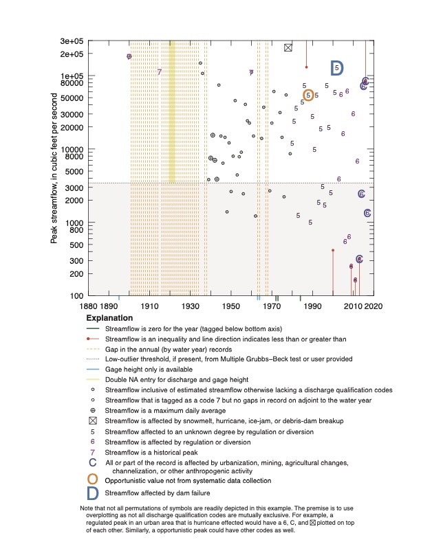
Author(s)

W.H. Asquith

References

U.S. Geological Survey, 2019, USGS water data for the Nation: U.S. Geological Survey National Water Information System database, accessed October 11, 2019, at doi:10.5066/F7P55KJN.

See Also

makeWaterYear, splitPeakCodes, plotFFQevol

Examples

## Not run: 
  # The dataRetrieval package is not required by MGBT algorithms.
  # Note that makeWaterYear() is not needed because splitPeakCodes() requires
  # the water_yr for gap analyses, and will call makeWaterYear() if it needs to.
  PK <- dataRetrieval::readNWISpeak("08167000", convertType=FALSE)
  PK <- splitPeakCodes(makeWaterYear(PK))
  plotPeaks(PK, codes=TRUE, showGHyrs=FALSE, site="08167000",
                xlab="Water year", ylab="Discharge, cfs") # 
## End(Not run)

## Not run: 
  # The dataRetrieval package is not required by MGBT algorithms.
  # An example with zero flows
  PK <- dataRetrieval::readNWISpeak("07148400", convertType=FALSE)
  PK <- splitPeakCodes(PK)
  plotPeaks(PK, codes=TRUE,  showDubNA=TRUE, site="07148400",
                xlab="Water year", ylab="Discharge, cfs") # 
## End(Not run)

## Not run: 
  # The dataRetrieval package is not required by MGBT algorithms.
  PK <- dataRetrieval::readNWISpeak("08329935", convertType=FALSE)
  PK <- splitPeakCodes(PK)
  plotPeaks(PK, codes=TRUE, showDubNA=TRUE, site="08329935",
                xlab="Water year", ylab="Discharge, cfs") # 
## End(Not run)

## Not run: 
  PK <- dataRetrieval::readNWISpeak("02146285", convertType=FALSE)
  PK <- splitPeakCodes(PK, all_peaks_na_okay=TRUE)
  plotPeaks(PK, site="02146285") # see likely message about all
  # peaks being missing assume that this streamgage forevermore
  # is a gage-height only site 
## End(Not run)

## Not run: 
  PK <- dataRetrieval::readNWISpeak("02317600", convertType=FALSE)
  PK <- splitPeakCodes(PK, all_peaks_na_okay=TRUE)
  plotPeaks(PK, site="02317600") 
## End(Not run)

Plot for More than One Streamgage that Peak Streamflows with Emphasis on Peak Discharge Qualification Codes

Description

Plot U.S. Geological Survey peak streamflows for multiple streamgages. This function is a wrapper on calls to plotPeaks with data retrieval occurring just ahead.

Usage

plotPeaks_batch(sites, file=NA, do_plot=TRUE,
                       silent=FALSE, envir=NULL, ...)

Arguments

Value

A list is returned by streamgage of the retrieved data with an attribute empty_sites storing those site numbers given for which no peaks were retrieved/processed. The data structure herein recognizes a NA for a site.

Author(s)

W.H. Asquith

References

U.S. Geological Survey, 2019, USGS water data for the Nation: U.S. Geological Survey National Water Information System database, accessed October 11, 2019, at doi:10.5066/F7P55KJN.

See Also

plotPeaks

Examples

## Not run: 
  # The dataRetrieval package is not required by MGBT algorithms, but needed
  # for the the plotPeaks_batch() function.
  sites <- c("07358570", "07358280", "07058980", "07258000")
  PK <- plotPeaks_batch(sites, xlab="WATER YEAR",         lot=0,
                               ylab="STREAMFLOW, IN CFS", file=NA) # 
## End(Not run)

## Not run: 
  # In this example, two calls to plotPeaks_batch() are made. The first is to use
  # the function as a means to cache the retrieval of the peaks without the
  # plotting overhead etc. The second is to actually perform the plotting.
  pdffile <- tempfile(pattern = "peaks", tmpdir = tempdir(), fileext = ".pdf")
  sites <- c("08106300", "08106310", "08106350", "08106500") # 08106350 no peaks

  PK <- plotPeaks_batch(sites, do_plot=FALSE)    # a hack to use its wrapper on
  # dataRetrieval::readNWISpeak() to get the peaks retrieved and code parsed by
  # splitPeakCodes() and then we can save the PK for later purposes as needed.

  empty_sites <- attr(PK, "empty_sites") # we harvest 08106350 as empty
  message("EMPTY SITES: ", paste(empty_sites, collapse=", "))

  PK <- as.environment(PK) # now flipping to environment for the actually plotting
                           # plotting pass to follow next and retrieval is not made
  # save(empty_sites, PK, file="PEAKS.RData") # a way to save the work for later
  PK <- plotPeaks_batch(sites, xlab="WATER YEAR",        lot=0, envir=PK,
                               ylab="STREAMFLOW, IN CFS", file=pdffile)
  message("Peaks plotted in file=", pdffile) # 
## End(Not run)

Relations Between Peak Streamflows to 1-Day Annual Maxima

Description

Both daily mean streamflow and instantaneous peak streamflows for many U.S. Geological Survey streamgages are available within the National Water Information System (NWIS). Peak streamflows are aggregated by water year (October 1 to September 30) NWIS and such streamflows are especially useful for flood frequency computations. Daily mean streamflows can be processed on a water year basis and 1-day annual maxima computed, and these maxima represent a 1-day volume as it were and are useful for flood volume frequency computations.

By strict definition, peak streamflows must equal or exceed 1-day annual maxima. Further 1-day annual maxima themselves should also underestimate a true volume maxima because a 1-day time step (midnight to midnight) is not a moving 24-hour or finer time-step resolution through streamflow hydrographs. Therefore, there are two mechanisms for 1-day maxima to be lesser than the peaks.

If a watershed is very large, flood hydrographs can be expected to be temporally wide and slow changing, such situations might have peak and 1-day annual maxima effectively equal to each other. Alternatively, if watershed is very small, flood hydrographs can be expected to be temporally of short duration and the peaks much larger than the 1-day annual maxima.

In terms of frequency computations, the peaks represent one dataset and the 1-day annual maxima another. There is not a restriction that the 1-day annual maxima be contemporaneously timed with the peak; although the hydrograph producing the peak is often aligned with maximum volume. The computations described herein consider the peak and the 1-day annual maxima to be simply distinct events and no processing of contemporaneousness is made aside from the simple water year designation.

This function supports optional caching of daily streamflow values and the peak streamflow values by environment keyed on the streamflow identification number. If a given cache is not provided, then the retrieval of the daily and (or) peak data are made using the dataRetrieval package. For the daily value cache, simply a data frame is needed of the Date and Flow columns from a previous or similar operation of the dataRetrieval::readNWISdv() function. For the peak value cache, simply a data frame from a previous operation of dataRetrieval::readNWISpeak() function is needed. The peak table internally is processed through splitPeakCodes to isolate peak streamflows by water year that appear to be part of systematic data collection activities. So called “opportunistic” peaks are ignored, but so-called “historical” peaks might be retained if the record appears as systematic.

Usage

ratioPeakMax1Day(siteNumber, dvenv=NULL, pkenv=NULL, as.list=FALSE,
                 missing.days=0, rm.ratios.lt1=TRUE, silent=TRUE, ...)

Arguments

Value

An R data.frame (the “ratio table”) is returned for a false as.list:

See Also

splitPeakCodes

Examples

## Not run: 
  site <- "08062700" # Example of 1980 peak being lower than 1-day maxima.
  D <- ratioPeakMax1Day(site, missing.days=0, rm.ratios.lt1=FALSE)
  print(D[D$ratio < 1,]) # 1980 on 18 Sep 2024 retrieval tests #
## End(Not run)

## Not run: 
  # site <- "08019200" # Example of peaks and maxima nearly identical.
    site <- "08167000" # Example of peaks and maxima being quite different.
  D <- ratioPeakMax1Day(site, missing.days=7) # permit a week of missing
  if(class(D) == "list") D <- D$ratios # if user added as.list=TRUE to call
  por <- paste0(min(D$water_yr), "-", max(D$water_yr),
                 " (", nrow(D), " processed water years)")
  plot(D$mx1d_flow, D$peak_flow, pch=21, col="black", bg="white", log="xy",
       xlab="Water year 1-day annual maxima streamflow, in cfs",
       ylab="Water year annual peak streamflow, in cfs")
  abline(0, 1); mtext(site, line=0.25)
  legend("topleft",    "Equal value line", bty="n", lty=1, pch=NA)
  legend("bottomright", por,               bty="n", lty=0, pch=NA)

  # Continuing, consider the two data sets via their order statistics, with us also
  # breaking the joint water year coupling in some study
  peakQ <- sort( log10(D$peak_flow) ) # order statistics of the peaks
  mx1dQ <- sort( log10(D$mx1d_flow) ) # order statistics of the maxima
  # let us for demonstration purposes only, use a log-normal distribution
  # and hence the use of log10() in the previous two calls
  peak_mu <- mean( peakQ ); peak_sd <- sd( peakQ ) # mean + std deviation
  mx1d_mu <- mean( mx1dQ ); mx1d_sd <- sd( mx1dQ ) # mean + std deviation

  FF <- seq(0.005, 0.995, by=0.005) # nonexceedances for drawing curves
  qFF <- qnorm(FF) # standard normal variates to transform x-axis
  peakPP  <- rank(peakQ) / (length(peakQ) + 1) # Weibull plotting position
  mx1dPP  <- rank(mx1dQ) / (length(mx1dQ) + 1) # Weibull plotting position
  peakFFQ <- 10^qnorm(FF, mean=peak_mu, sd=peak_sd) # Log-normal curves
  mx1dFFQ <- 10^qnorm(FF, mean=mx1d_mu, sd=mx1d_sd) # Log-normal curves

  ylim <- range(c(1, peakQ / mx1dQ, log10(D$peak_flow) / log10(D$mx1d_flow)))
  x <- log10(D$mx1d_flow);     y <- log10(D$peak_flow) / log10(D$mx1d_flow)
  plot(mx1dQ, peakQ / mx1dQ, type="l", col="darkgreen", pch=21, bg="lightgreen",
       xlab="log10(water year 1-day annual maxima streamflow)", ylim=ylim, las=1,
       ylab="Ratio of annual peak to 1-day annual maxima")
  lines(x[order(x)], y[order(x)], pch=23, col="salmon4",   bg="salmon1"   )
  points(mx1dQ, peakQ / mx1dQ,    pch=21, col="darkgreen", bg="lightgreen", cex=1.3)
  points(log10(D$mx1d_flow), log10(D$peak_flow) / log10(D$mx1d_flow),
         pch=23, col="salmon4", bg="salmon1", cex=0.8)
  txt <- c("Joint ratio by separate sorting of peak and annual maxima",
           "Ratio by maintaining water year as the connection")
  legend("bottomright", txt, cex=0.8, bty="n", pch=c(21, 23), lty=c(1, 1), bg="white",
         col=c("darkgreen", "salmon4"), pt.cex=1, pt.bg=c("lightgreen", "salmon1"))
  mtext(site, line=0.25)

  plot(qnorm(FF), peakFFQ, type="n", log="y",
       ylim=range(c(10^peakQ, 10^mx1dQ, peakFFQ, mx1dFFQ)),
       xlab="Standard normal variate", ylab="Flood magnitude, in cfs")
  points(qnorm(peakPP), 10^peakQ, pch=21, col="red",  bg="white")
  points(qnorm(peakPP), 10^mx1dQ, pch=22, col="blue", bg="white")
  lines(qFF, peakFFQ, col="red",  lty=2); lines(qFF, mx1dFFQ, col="blue", lty=2)
  txt <- c("Peak streamflow frequency to data shown",
           "1-day annual maxima frequency to data shown",
           "Observed annual peak streamflow",
           "Observed 1-day annual maxima streamflow")
  legend("topleft", txt, bty="n", lty=c(2, 2, NA, NA), bg="white",
          pch=c(NA, NA, 21, 22), col=c("red", "blue", "red", "blue"))
  mtext(site, line=0.25) # 
## End(Not run)

## Not run: 
  # Continuation of the previous dontrun{} block, we now try to "use" the ratio by
  # imagining what flood frequency would look like without having the peaks themselves.
  # The context is to imagine streamflow data stemming from nonUSGS streamflow sources
  # and there are no peaks available. Perhaps one could study analog watersheds of the
  # USGS and create a statistical model to predict a correction of the 1-day to the
  # peaks based on watershed properties and derived pseudo-peaks. First two "obvious"
  # ways to look at the peak to maxima ratios by means of the ratios:
  phi_simpl <-    mean(D$ratio)                                      # arithmetic
  phi_geomu <- cumprod(D$ratio)[length(D$ratio)]^(1/length(D$ratio)) # geometric

  # Then, let us think about the coupling between the two datasets by their order
  # statistics. This is potentially more informative because structurally the frequency
  # curves themselves derived in some methods from the order statistics (L-moments or
  # product spacings).
  phi_infor <- mean(peakQ / mx1dQ) # mean ratio of the log10 flows
  phi_log10 <- mean(D$log10diff)   # mean log10 offset (phi_geomu == 10^phi_log10)

  # Continuing with simple log-normal distribution model, now correct maxima
  mx1d_mu_simpl <- mean( log10( phi_simpl * 10^mx1dQ ) )
  mx1d_sd_simpl <-   sd( log10( phi_simpl * 10^mx1dQ ) )
  mx1dFFQ_simpl <- 10^qnorm(FF, mean=mx1d_mu_simpl, sd=mx1d_sd_simpl)
  # Correct maxima by goemetric mean
  mx1d_mu_geomu <- mean( log10( phi_geomu * 10^mx1dQ ) )
  mx1d_sd_geomu <-   sd( log10( phi_geomu * 10^mx1dQ ) )
  mx1dFFQ_geomu <- 10^qnorm(FF, mean=mx1d_mu_geomu, sd=mx1d_sd_geomu)
  mx1dFFQ_log10 <- 10^(  log10(mx1dFFQ) + phi_log10  ) # This is the same as if
  # the geometric mean were used as shown for mx1dFFQ_geomu. It seems more concise
  # to think of a simple log10 offset than geometric mean.

  # Now, consider relative variation as a constant and therefore the variation
  # (standard deviation) likely needs some scaling as well. We use the CV of the
  # original sample and after the mean is rescaled, the standard deviation is too.
  cv <- sd( mx1dQ ) / mean( mx1dQ ) # coefficient of variation (CV)
  mx1d_mu_infor <- mean( mx1dQ ) *     phi_infor
  mx1d_sd_infor <-            cv * mx1d_mu_infor
  mx1dFFQ_infor <- 10^qnorm(FF, mean=mx1d_mu_infor, sd=mx1d_sd_infor)

  cols <- c("red", "blue", "turquoise3", "purple", "palegreen4", "red", "blue")
  plot(qnorm(FF), peakFFQ, type="n", log="y",
       ylim=range(c(10^peakQ, 10^mx1dQ, peakFFQ, mx1dFFQ)),
       xlab="Standard normal variate", ylab="Flood magnitude, in cfs")
  points(qnorm(peakPP), 10^peakQ, pch=21, col=cols[1], bg="white", lty=2)
  points(qnorm(peakPP), 10^mx1dQ, pch=21, col=cols[2], bg="white", lty=2)
  lines(qFF, peakFFQ, col=cols[1], lty=2); lines(qFF, mx1dFFQ, col=cols[2], lty=2)
  lines(qFF, mx1dFFQ_simpl, col=cols[3], lwd=2)
  lines(qFF, mx1dFFQ_log10, col=cols[4], lwd=2)
  lines(qFF, mx1dFFQ_infor, col=cols[5], lwd=3)
  legend("topleft", c("Peak streamflow frequency to data shown",
   "1-day annual maxima frequency to data shown", "Pseudo-peak frequency by mean-ratio",
   "Pseudo-peak frequency by log10-offset", "Pseudo-peak frequency by mean-cv-logratio",
   "Observed annual peak streamflow", "Observed 1-day annual maxima streamflow"),
         bty="n", pch=c(NA, NA, NA, NA, NA, 21, 21), pt.cex=1, bg="white",
         lwd=c(1, 1, 2, 2, 3, NA, NA), lty=c(2, 2, 1, 1, 1, NA, NA), col=cols)
  mtext(site, line=0.25) # 
## End(Not run)

Read NWIS WATSTORE-Formatted Period of Record Peak Streamflows and Other Germane Operations

Description

Read U.S. Geological Survey (USGS) National Water Information System (NWIS) (U.S. Geological Survey, 2019) peak streamflows. But with a major high-level twist what is retained or produced by the operation. This function retrieves the WATSTORE formatted version of the peak streamflow data on a streamgage by streamgage basis and this is the format especially suitable for the USGS PeakFQ software (U.S. Geological Survey, 2020). That format will reflect the period of record. This function uses direct URL pathing to NWIS to retrieve this format and write the results to the user's file system. The function does not use the dataRetrieval package for the WATSTORE format. Then optionally, this function uses the dataRetrieval package to retrieve a tab-delimited version of the peak streamflows and write those to the user's file system. Peak streamflow visualization with attention to the peak discharge qualification codes and other features is optionally made here by the plotPeaks function and optionally a portable document formatted graphics file can be written as well. This function is explicitly design around a single directory for each streamgage to store the retrieved and plotted data.

Usage

readNWISwatstore(siteNumbers, path=".", dirend="d", return.progress=FALSE,
                              tabpk=TRUE, vispk=TRUE, vispdf=TRUE,
                              unlinkpath=FALSE, citeNWISdoi=TRUE,
                              all_peaks_na_okay=TRUE, ...)

Arguments

Value

No values are returned; this function is used for its file system side effects. Those effects will include ".pkf" (WATSTORE formatted peak streamflow data) and potentially include the following additional file by extension: ".pdf", ".txt" (tab-delimited peak streamflow data), and CITATION.md file recording a correct policy-compliant citation to the USGS NWIS DOI number with access date as per additional arguments to this function. This function does not recognize the starting and ending period options that the dataRetrieval package provides because the WATSTORE format is ensured to be period of record. Therefore, the disabling of optional period retrievals ensures that the ".pkf" and ".[txt|pdf]" files have the same data.

Author(s)

W.H. Asquith

References

U.S. Geological Survey, 2019, USGS water data for the Nation: U.S. Geological Survey National Water Information System database, accessed October 11, 2019, at doi:10.5066/F7P55KJN.

U.S. Geological Survey, 2020, PeakFQ—Flood frequency analysis based on Bulletin 17C and recommendations of the Advisory Committee on Water Information (ACWI) Subcommittee on Hydrology (SOH) Hydrologic Frequency Analysis Work Group (HFAWG), version 7.3.

See Also

plotPeaks

Examples

## Not run: 
  # The dataRetrieval package provides a readNWISpeak() function but that works on
  # the tab-delimited like format structure and not the WATSTORE structure. The
  # WATSTORE structure is used by the USGS PeakFQ software and direct URL is needed
  # to acquire such data
  path <- tempdir()
  readNWISwatstore("08167000", path=path)
  # path/08167000d/08167000.[pdf|pkf|txt]
  #                CITATION.md
  # files will be created in the temporary directory 
## End(Not run)

## Not run: 
  # a gage-height only site, table created, codes split, and then the plot so
  # produced is produced with a message in the middle about all peaks missing
  readNWISwatstore("02146285", path=tempdir(), dirend="d",
            tabpk=TRUE, vispk=TRUE, vispdf=TRUE, unlinkpath=FALSE,
            citeNWISdoi=TRUE, all_peaks_na_okay=TRUE) # 
## End(Not run)

## Not run: 
  sites <- c("08171000", "02231100", "02317600")
  gotEM <- readNWISwatstore(sites, path=tempdir(),
                            return.progress=TRUE, unlinkpath=FALSE)
  # WHA On January 23, 2023, we see first this message from dataRetrieval:
  # No sites/data found using the selection criteria specified
  # WHA then readNWISwatstore() then adds clarity on which streamgage failed
  #   for streamgage '02231100'
  # WHA because this streamgage does not have any peaks entries and appears to be a
  # WHA measurement only site. The readNWISwatstore() continues and the following
  # WHA warnings occur
  # Warning messages:
  # 1: In makeWaterYear(x) : water year 2019 occurs more than once (x2)
  # 2: In plotPeaks2(pkall, codes = TRUE, showDubNA = TRUE, site = site,  :
  # site '02317600', water year 2019 occurs more than once (x2) (drawing them all)
  # WHA because streamgage 02317600 has two records that process into the 2019
  # WHA water years, which technically is not possible with annual maxima series.
  head(gotEM)
  #      site gotThePeaks
  # 1 08171000        TRUE # successful retrieval w/o identified problems
  # 2 02231100       FALSE # no peak records to retrieve
  # 3 02317600        TRUE # records retrieved but the 2019 water year is duplicated 
## End(Not run)

Split the Peak Discharge Qualifications Codes into Separate Columns

Description

Split the U.S. Geological Survey (USGS) peak discharge qualifications codes (Asquith and others, 2017; U.S. Geological Survey, 2021) in the peak_cd column of a peak-streamflow data retrieval from the USGS National Water Information System (NWIS) (U.S. Geological Survey, 2019) in a data.frame into separate columns of the input data.frame. The NWIS system stores all the codes within a single database field. It can be useful for graphical (plotPeaks) or other statistical study to have single logical variable for each of the codes, and such is the purpose of this function. Note because of the appearsSystematic field is based computations involving the water_yr (water year), this function needs the makeWaterYear to have been run first; however, the function will autodetect and call that function internally if needed and those effects are provided on the returned data.frame. (See also plotPeaks; see also the inst/legend/ subdirectory of this package for a script to produce a legend as well as inst/legend/legend_camera.pdf, which has been dressed up in a vector graphics editing program.)

Usage

splitPeakCodes(x, all_peaks_na_okay=FALSE)

Arguments

Value

The x as originally inputted is returned with the addition of these columns:

Note

Concerning appearsSystematic: All records but missing discharges are assumed as systematic records unless the peak streamflows are missing or peaks have a code 7 but there are existing years on either side of individual peaks coded as 7. The logic also handles a so-called “roll-on” and “roll-off” of the data by only testing the leading or trailing year—except this becomes a problem if multiple stations are involved, so the code will return early with a warning. Importantly, it is possible that some code 7s can be flagged as systematic and these are not necessarily in error. Testing indicates that some USGS Water Science Centers (maintainers of databases) have historically slightly different tendencies in application of the code 7. The USGS NWIS database does not actually contain a field indicating that a peak was collected as part of systematic operation and hence that peak is part of an assumed random sample. Peaks with gage height only are flagged as nonsystematic by fiat—this might not be the best solution over all, but because virtually all statistics use the discharge column this seems okay (feature is subject to future changes).

Concerning anyCodes, only the regular expression A|B|C|D|O|1|2|3|4|5|6|7|8|9 will trigger setting anyCodes to TRUE. For example, it is felt that codes E, F, and R are basically meaningless for statistic study and do not represent the “special circumstances” of information as reflected in the aforementioned list of others codes. The codes Bd and Bm are uninformative too and the column appending by makeWaterYear accommodates the necessary structure for further study of date precision if needed by a developer.

A comprehensive listing of peak codes (peak_cd) and peak gage heights (gage_cd) follows (U.S. Geological Survey, 2021):

peak_cd
  1	----> Discharge is a Maximum Daily Average
  2	----> Discharge is an Estimate
  3	----> Discharge affected by Dam Failure
  4	----> Discharge less than indicated value which is Minimum Recordable
            Discharge at this site
  5	----> Discharge affected to unknown degree by Regulation or Diversion
  6	----> Discharge affected by Regulation or Diversion
  7	----> Discharge is an Historic Peak
  8	----> Discharge actually greater than indicated value
  9	----> Discharge due to Snowmelt, Hurricane, Ice-Jam or Debris Dam breakup
  A	----> Year of occurrence is unknown or not exact
 Bd	----> Day of occurrence is unknown or not exact
 Bm	----> Month of occurrence is unknown or not exact
  C	----> All or part of the record affected by Urbanization, Mining,
            Agricultural changes, Channelization, or other
  D	----> Base Discharge changed during this year
  E	----> Only Annual Maximum Peak available for this year
  F	----> Peak supplied by another agency
  O	----> Opportunistic value not from systematic data collection
  R	----> Revised

gage_cd
  1	----> Gage height affected by backwater
  2	----> Gage height not the maximum for the year
  3	----> Gage height was at a different site and/or datum
  4	----> Gage height below minimum recordable elevation
  5	----> Gage height is an estimate
  6	----> Gage height datum changed during this year
  7	----> Debris, mud, or hyper-concentrated flow
  8	----> Gage height tidally affected
 Bd	----> Day of occurrence is unknown or not exact
 Bm	----> Month of occurrence is unknown or not exact
  F	----> Peak supplied by another agency
  R	----> Revised

The authors of the MGBT package want to make a remark that the code 4 in many parts of the United States might not reflect the complete idea of “which is minimum recordable discharge at this site.” More generally, the code 4 should be thought of a censoring flag for a “less then discharge” (Asquith and others, 2018). There are streamgages that in theory could be recording zero to infinite discharge, but then when information is compiled for the year, the annual peak might be flagged as a less than some threshold and have no bearing on the idea of a minimum recordable for the streamgage itself. Such a situation could stem from multiple gage height recording apparatus measuring culvert-like flow circumstances (Asquith and others, 2018).

Author(s)

W.H. Asquith

References

Asquith, W.H., Harwell, G.R., and Winters, K.E., 2018, Annual and approximately quarterly series peak streamflow derived from interpretations of indirect measurements for a crest-stage gage network in Texas through water year 2015: U.S. Geological Survey Scientific Investigations Report 2018–5107, 24 p., doi:10.3133/sir20185107.

Asquith, W.H., Kiang, J.E., and Cohn, T.A., 2017, Application of at-site peak-streamflow frequency analyses for very low annual exceedance probabilities: U.S. Geological Survey Scientific Investigation Report 2017–5038, 93 p., doi:10.3133/sir20175038.

U.S. Geological Survey, 2019, USGS water data for the Nation: U.S. Geological Survey National Water Information System database, accessed October 11, 2019, at doi:10.5066/F7P55KJN.

U.S. Geological Survey, 2021, Peak Streamflow and Stage Special Conditions (PEAK.peak_cd and PEAK.gage_ht_cd).

See Also

makeWaterYear, plotPeaks

Examples

## Not run: 
  # The dataRetrieval package is not required by MGBT algorithms.
  PK <- dataRetrieval::readNWISpeak("08167000", convertType=FALSE)
  PK <- splitPeakCodes(PK)
  names(PK) # See that the columns are there.
## End(Not run)